Chapter 39 Dealing with Missing Data
So what we should have done at the start of our wcgs analysis was to identify any issues with missing values or whether any variables show unreasonably large or small values.
39.1 Identifying Missingness
If you just want a count of missing values, you can use colSums and is.na
   id  chol   age   bmi   sbp   dbp smoke
    0    12     0     0     0     0     0
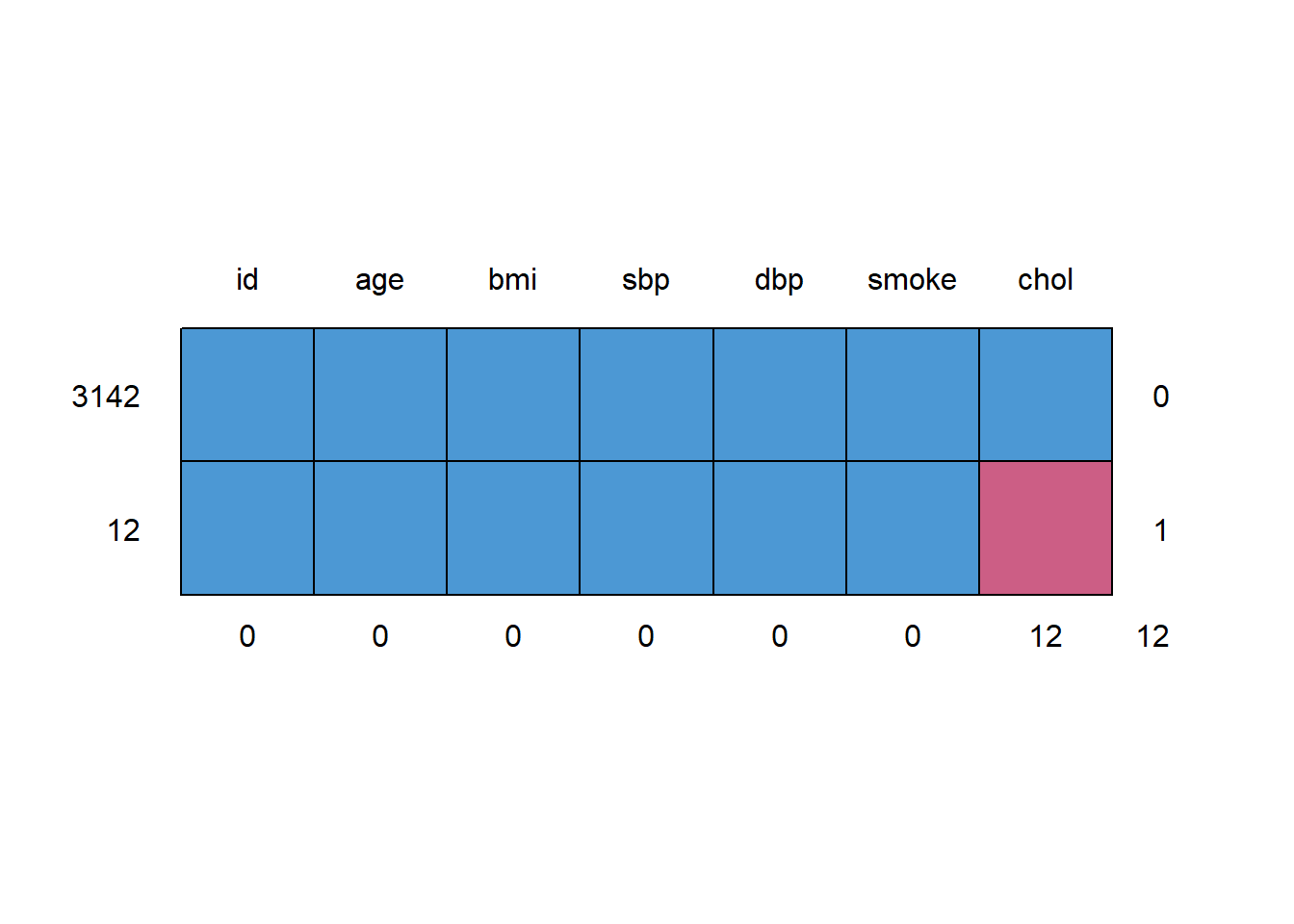
The mice package provides the md.pattern function to identify missingness patterns.

     id age bmi sbp dbp smoke chol
3142  1   1   1   1   1     1    1  0
12    1   1   1   1   1     1    0  1
      0   0   0   0   0     0   12 12
Given the relatively small set of variables we’re studying here, I would run the describe function from the Hmisc package on each variable (maybe skipping id) in order to identify missing and (potentially) unrealistic values through range checks.
wcgs.s[-1]

 6  Variables      3154  Observations
---------------------------------------------------------------------------
chol
       n  missing distinct     Info     Mean      Gmd      .05      .10
    3142       12      237        1    226.4    47.99    161.1    175.0
     .25      .50      .75      .90      .95
   197.2    223.0    253.0    280.0    302.0

lowest : 103 110 111 112 113, highest: 386 390 400 414 645
---------------------------------------------------------------------------
age
       n  missing distinct     Info     Mean      Gmd      .05      .10
    3154        0       21    0.996    46.28    6.256       39       40
     .25      .50      .75      .90      .95
      42       45       50       55       57

lowest : 39 40 41 42 43, highest: 55 56 57 58 59
---------------------------------------------------------------------------
bmi
       n  missing distinct     Info     Mean      Gmd      .05      .10
    3154        0      679        1    24.52    2.803    20.59    21.52
     .25      .50      .75      .90      .95
   22.96    24.39    25.84    27.45    28.73

lowest : 11.2 15.7 16.9 17.2 17.2, highest: 36.0 37.2 37.2 37.7 38.9
---------------------------------------------------------------------------
sbp
       n  missing distinct     Info     Mean      Gmd      .05      .10
    3154        0       62    0.996    128.6    16.25      110      112
     .25      .50      .75      .90      .95
     120      126      136      148      156

lowest :  98 100 102 104 106, highest: 200 208 210 212 230
---------------------------------------------------------------------------
dbp
       n  missing distinct     Info     Mean      Gmd      .05      .10
    3154        0       42    0.992    82.02    10.51       68       70
     .25      .50      .75      .90      .95
      76       80       86       94      100

lowest :  58  60  62  64  66, highest: 125 129 130 136 150
---------------------------------------------------------------------------
smoke
       n  missing distinct
    3154        0        2

Value         No   Yes
Frequency   1652  1502
Proportion 0.524 0.476
---------------------------------------------------------------------------
No values are outside the range of plausibility, and in any case, we see that we have 12 missing chol values in the full data set. Options?
- We might choose to omit those rows before creating our test and training samples.
- If we’re building a model where
cholis the outcome, I would omit those cases, as (for 431, at least) I won’t impute outcomes. This is R’s default.
- If we’re building a model where
- We might choose to impute missing values after we partition.
39.2 Complete Case Analysis: A model for chol
Suppose we want to build a model for chol using age, body-mass index and systolic blood pressure, using the entire wcgs data frame, except those subjects with a missing chol value. Note that this is the default approach R takes, regardless of whether chol is used as an outcome or predictor.
Call:
lm(formula = chol ~ age + bmi + sbp, data = wcgs.s)

Residuals:
   Min     1Q Median     3Q    Max
-125.4  -28.6   -3.0   25.9  409.4

Coefficients:
            Estimate Std. Error t value Pr(>|t|)
(Intercept)  146.871     10.320   14.23  < 2e-16 ***
age            0.561      0.141    3.98  7.2e-05 ***
bmi            0.681      0.312    2.18    0.029 *
sbp            0.287      0.054    5.31  1.2e-07 ***
---
Signif. codes:  0 '***' 0.001 '**' 0.01 '*' 0.05 '.' 0.1 ' ' 1

Residual standard error: 43 on 3138 degrees of freedom
  (12 observations deleted due to missingness)
Multiple R-squared:  0.0214,    Adjusted R-squared:  0.0205
F-statistic: 22.9 on 3 and 3138 DF,  p-value: 1.16e-14
The notification under the residual standard error indicates that 12 observations (the 12 with missing chol, since no other variables in this group have missing data) were dropped before the model was fit. You can also tell this from the degrees of freedom.
- We have four coefficients to fit (intercept and slopes of
age,bmiandsbp) so we have (4 - 1) = 3 numerator degrees of freedom. - The ANOVA F-statistic report also specifies 3138 denominator degrees of freedom.
- Total df is always one less than the total number of observations used in the model.
- That suggests we are using (3 + 3138) + 1 = 3142 subjects in this model.
- But
wcgs.sactually contains 3,154 people so 12 were omitted.
[1] 3154 739.2.1 Removing all subjects with NA, via na.omit
So, if we want to fit a complete case analysis, we don’t, technically, have to do anything except specify the model. We can also make this explicit by first pruning all subjects with any missing values on any variables from our tibble.
wcgs.subnoNA <- dplyr::select(wcgs, id, chol, age, bmi, sbp) %>%
    na.omit ## the na.omit function drops all cases with NA
dim(wcgs.subnoNA)
[1] 3142 539.2.2 Removing subjects with NA on one particular variable
If we wanted to specify that only subjects with missing chol should be removed from the data set (in case there were missing values in other variables), we could use the following approach.
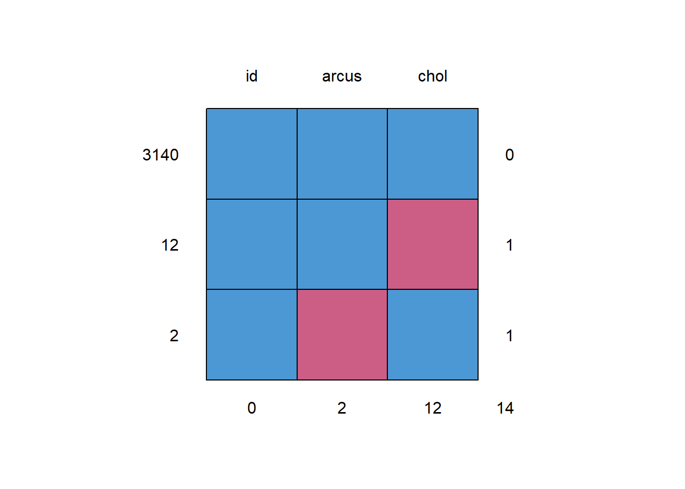
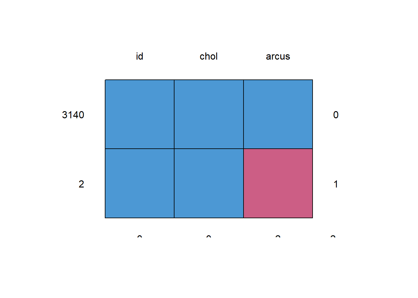
Here, I’ll work with a data set (wcgs.s3) that contains 12 missing chol values, and 2 missing arcus values, and build a new set (wcgs.s3noNAchol) that retains the subjects who have a chol value, regardless of whether they are also missing arcus, but not include the 12 subjects with missing chol data

     id arcus chol
3140  1     1    1  0
12    1     1    0  1
2     1     0    1  1
      0     2   12 14
     id chol arcus
3140  1    1     1 0
2     1    1     0 1
      0    0     2 2
39.3 Using Multiple Imputation to fit our Regression Model
Following the approach we outlined in the R-20 document, we’ll try fitting the model while imputing the 12 cholesterol values, 100 times each, creating 100 new “complete” data sets.
wcgs.sub <- wcgs %>% dplyr::select(id, chol, age, bmi, sbp)
chol.mi <- mice(wcgs.sub, m = 100, maxit = 5,
                meth = "pmm", printFlag = FALSE, seed = 4314)
39.3.1 Examining a Single Imputed Data Set
We could look at any one of our 100 imputations in some detail, perhaps the 12th such imputation, as follows:
imp12$chol
       n  missing distinct     Info     Mean      Gmd      .05      .10
    3154        0      237        1    226.4    47.98    161.7    175.0
     .25      .50      .75      .90      .95
   197.2    223.0    253.0    280.0    302.0

lowest : 103 110 111 112 113, highest: 386 390 400 414 645
Working with a particular imputation might allow us to produce plots of the imputed data, or of diagnostics after a regression model, but we’ll focus our interpretation of regression results (in 431) on estimates of coefficients and of things like R2. For that, we want to use all 100 imputations, in a pooled approach.
39.3.2 Fitting a Pooled Regression Model across the Imputations
Next, we’ll fit a set of pooled regression model estimates across all 100 imputations, producing the following results. We’ll even estimate both forms of R2.
Class: mipo    m = 100
            estimate     ubar        b        t dfcom   df     riv  lambda
(Intercept)  146.993 1.06e+02 8.02e-01 1.07e+02  3150 3118 0.00766 0.00760
age            0.563 1.97e-02 1.47e-04 1.99e-02  3150 3119 0.00752 0.00747
bmi            0.685 9.69e-02 7.06e-04 9.76e-02  3150 3120 0.00735 0.00730
sbp            0.284 2.87e-03 4.84e-05 2.92e-03  3150 3068 0.01702 0.01674
                fmi
(Intercept) 0.00823
age         0.00810
bmi         0.00794
sbp 0.01738 estimate std.error statistic df p.value
(Intercept) 146.99 10.33 14.23 3118 0.00
age 0.56 0.14 3.99 3119 0.00
bmi 0.69 0.31 2.19 3120 0.03
sbp 0.28 0.05 5.25 3068 0.00 est lo 95 hi 95 fmi
R^2 0.0214 0.0125 0.0325 NaN est lo 95 hi 95 fmi
adj R^2 0.0204 0.0118 0.0314 NaNfmiin the output above contains the fraction of missing information.lambdain that output is the proportion of the total variance that is attributable to the missing data.
So, how do these estimates after imputation compare to our complete case analysis originally developed as model1, and re-summarized below?
Call:
lm(formula = chol ~ age + bmi + sbp, data = wcgs.s)

Residuals:
   Min     1Q Median     3Q    Max
-125.4  -28.6   -3.0   25.9  409.4

Coefficients:
            Estimate Std. Error t value Pr(>|t|)
(Intercept)  146.871     10.320   14.23  < 2e-16 ***
age            0.561      0.141    3.98  7.2e-05 ***
bmi            0.681      0.312    2.18    0.029 *
sbp            0.287      0.054    5.31  1.2e-07 ***
---
Signif. codes:  0 '***' 0.001 '**' 0.01 '*' 0.05 '.' 0.1 ' ' 1

Residual standard error: 43 on 3138 degrees of freedom
  (12 observations deleted due to missingness)
Multiple R-squared:  0.0214,    Adjusted R-squared:  0.0205
F-statistic: 22.9 on 3 and 3138 DF,  p-value: 1.16e-14
39.4 Comparing Two Models After Imputation with pool.compare
Suppose we want to assess whether a model for chol with age, bmi and sbp is statistically significantly more effective than a model with age alone. As long as the models we want to compare are nested (so that one model is a proper subset of the other), then this can be done as follows, to produce a Wald test.
model.1mi <- with(chol.mi, lm(chol ~ age + bmi + sbp))
model.2mi <- with(chol.mi, lm(chol ~ age))
comp1 <- pool.compare(model.1mi, model.2mi, method = "wald")(Intercept) age bmi sbp
146.993 0.563 0.685 0.284 (Intercept) age
194.0 0.7 [,1]
[1,] 16.3[1] 2[1] 1311410 [,1]
[1,] 8.71e-08Practically, a significant value of the Wald test here suggests that the difference in predictive value between model.1mi and model.2mi is statistically significant, and thus, that you need the larger model. A non-significant Wald test would be consistent with a situation where you could use the model with age alone.
Here, we clearly want to retain bmi and sbp as compared to dropping them both from the model. This isn’t a surprise, as we saw previously that both bmi and sbp had apparent predictive value (by the t test) even after all other variables were already in the model.
To create the overall F test, we could compare our model to an intercept only model,
model.intmi <- with(chol.mi, lm(chol ~ 1)) but we’ll skip that here.