Chapter 2 Linear Regression on a small SMART data set

2.1 BRFSS and SMART

The Centers for Disease Control analyzes Behavioral Risk Factor Surveillance System (BRFSS) survey data for specific metropolitan and micropolitan statistical areas (MMSAs) in a program called the Selected Metropolitan/Micropolitan Area Risk Trends of BRFSS (SMART BRFSS.)

In this work, we will focus on data from the 2016 SMART, and in particular on data from the Cleveland-Elyria, OH, Metropolitan Statistical Area. The purpose of this survey is to provide localized health information that can help public health practitioners identify local emerging health problems, plan and evaluate local responses, and efficiently allocate resources to specific needs.

2.1.1 Key resources

• the full data are available in the form of the 2016 SMART BRFSS MMSA Data, found in a zipped SAS Transport Format file. The data were released in August 2017.
• the MMSA Variable Layout PDF which simply lists the variables included in the data file
• the Calculated Variables PDF which describes the risk factors by data variable names - there is also an online summary matrix of these calculated variables, as well.
• the lengthy 2016 Survey Questions PDF which lists all questions asked as part of the BRFSS in 2016
• the enormous Codebook for the 2016 BRFSS Survey PDF which identifies the variables by name for us.

Later this term, we’ll use all of those resources to help construct a more complete data set than we’ll study today. I’ll also demonstrate how I built the smartcle1 data set that we’ll use in this Chapter.

2.2 The smartcle1 data: Cookbook

The smartcle1.csv data file available on the Data and Code page of our website describes information on 11 variables for 1036 respondents to the BRFSS 2016, who live in the Cleveland-Elyria, OH, Metropolitan Statistical Area. The variables in the smartcle1.csv file are listed below, along with (in some cases) the BRFSS items that generate these responses.

Variable	Description
SEQNO	respondent identification number (all begin with 2016)
physhealth	Now thinking about your physical health, which includes physical illness and injury, for how many days during the past 30 days was your physical health not good?
menthealth	Now thinking about your mental health, which includes stress, depression, and problems with emotions, for how many days during the past 30 days was your mental health not good?
poorhealth	During the past 30 days, for about how many days did poor physical or mental health keep you from doing your usual activities, such as self-care, work, or recreation?
genhealth	Would you say that in general, your health is … (five categories: Excellent, Very Good, Good, Fair or Poor)
bmi	Body mass index, in kg/m2
female	Sex, 1 = female, 0 = male
internet30	Have you used the internet in the past 30 days? (1 = yes, 0 = no)
exerany	During the past month, other than your regular job, did you participate in any physical activities or exercises such as running, calisthenics, golf, gardening, or walking for exercise? (1 = yes, 0 = no)
sleephrs	On average, how many hours of sleep do you get in a 24-hour period?
alcdays	How many days during the past 30 days did you have at least one drink of any alcoholic beverage such as beer, wine, a malt beverage or liquor?

str(smartcle1)

Classes 'tbl_df', 'tbl' and 'data.frame':   1036 obs. of  11 variables:
 $ SEQNO     : num  2.02e+09 2.02e+09 2.02e+09 2.02e+09 2.02e+09 ...
 $ physhealth: int  0 0 1 0 5 4 2 2 0 0 ...
 $ menthealth: int  0 0 5 0 0 18 0 3 0 0 ...
 $ poorhealth: int  NA NA 0 NA 0 6 0 0 NA NA ...
 $ genhealth : Factor w/ 5 levels "1_Excellent",..: 2 1 2 3 1 2 3 3 2 3 ...
 $ bmi       : num  26.7 23.7 26.9 21.7 24.1 ...
 $ female    : int  1 0 0 1 0 0 1 1 0 0 ...
 $ internet30: int  1 1 1 1 1 1 1 1 1 1 ...
 $ exerany   : int  1 1 0 1 1 1 1 1 1 0 ...
 $ sleephrs  : int  6 6 8 9 7 5 9 7 7 7 ...
 $ alcdays   : int  1 4 4 3 2 28 4 2 4 25 ...

2.3 smartcle2: Omitting Missing Observations: Complete-Case Analyses

For the purpose of fitting our first few models, we will eliminate the missingness problem, and look only at the complete cases in our smartcle1 data. We will discuss methods for imputing missing data later in these Notes.

To inspect the missingness in our data, we might consider using the skim function from the skimr package. We’ll exclude the respondent identifier code (SEQNO) from this summary as uninteresting.

skim_with(numeric = list(hist = NULL), integer = list(hist = NULL))
## above line eliminates the sparkline histograms
## it can be commented out when working in the console,
## but I need it to produce the Notes without errors right now

smartcle1 %>% 
    skim(-SEQNO)

Skim summary statistics
 n obs: 1036 
 n variables: 11 

-- Variable type:factor -----------------------------------------------------------
  variable missing complete    n n_unique
 genhealth       3     1033 1036        5
                             top_counts ordered
 2_V: 350, 3_G: 344, 1_E: 173, 4_F: 122   FALSE

-- Variable type:integer ----------------------------------------------------------
   variable missing complete    n mean   sd p0 p25 p50 p75 p100
    alcdays      46      990 1036 4.65 8.05  0   0   1   4   30
    exerany       3     1033 1036 0.76 0.43  0   1   1   1    1
     female       0     1036 1036 0.6  0.49  0   0   1   1    1
 internet30       6     1030 1036 0.81 0.39  0   1   1   1    1
 menthealth      11     1025 1036 2.72 6.82  0   0   0   2   30
 physhealth      17     1019 1036 3.97 8.67  0   0   0   2   30
 poorhealth     543      493 1036 4.07 8.09  0   0   0   3   30
   sleephrs       8     1028 1036 7.02 1.53  1   6   7   8   20

-- Variable type:numeric ----------------------------------------------------------
 variable missing complete    n  mean   sd    p0  p25   p50   p75  p100
      bmi      84      952 1036 27.89 6.47 12.71 23.7 26.68 30.53 66.06

Now, we’ll create a new tibble called smartcle2 which contains every variable except poorhealth, and which includes all respondents with complete data on the variables (other than poorhealth). We’ll store those observations with complete data in the smartcle2 tibble.

smartcle2 <- smartcle1 %>% 
    select(-poorhealth) %>%
    filter(complete.cases(.))

smartcle2

# A tibble: 896 x 10
    SEQNO physhealth menthealth genhealth   bmi female internet30 exerany
    <dbl>      <int>      <int> <fct>     <dbl>  <int>      <int>   <int>
 1 2.02e9          0          0 2_VeryGo~  26.7      1          1       1
 2 2.02e9          0          0 1_Excell~  23.7      0          1       1
 3 2.02e9          1          5 2_VeryGo~  26.9      0          1       0
 4 2.02e9          0          0 3_Good     21.7      1          1       1
 5 2.02e9          5          0 1_Excell~  24.1      0          1       1
 6 2.02e9          4         18 2_VeryGo~  27.6      0          1       1
 7 2.02e9          2          0 3_Good     25.7      1          1       1
 8 2.02e9          2          3 3_Good     28.5      1          1       1
 9 2.02e9          0          0 2_VeryGo~  28.6      0          1       1
10 2.02e9          0          0 3_Good     23.1      0          1       0
# ... with 886 more rows, and 2 more variables: sleephrs <int>,
#   alcdays <int>

Note that there are only 896 respondents with complete data on the 10 variables (excluding poorhealth) in the smartcle2 tibble, as compared to our original smartcle1 data which described 1036 respondents and 11 variables, but with lots of missing data.

2.4 Summarizing the smartcle2 data numerically

2.4.1 The New Toy: The skim function

skim(smartcle2, -SEQNO)

Skim summary statistics
 n obs: 896 
 n variables: 10 

-- Variable type:factor -----------------------------------------------------------
  variable missing complete   n n_unique
 genhealth       0      896 896        5
                             top_counts ordered
 2_V: 306, 3_G: 295, 1_E: 155, 4_F: 102   FALSE

-- Variable type:integer ----------------------------------------------------------
   variable missing complete   n mean   sd p0 p25 p50 p75 p100
    alcdays       0      896 896 4.83 8.14  0   0   1   5   30
    exerany       0      896 896 0.77 0.42  0   1   1   1    1
     female       0      896 896 0.58 0.49  0   0   1   1    1
 internet30       0      896 896 0.81 0.39  0   1   1   1    1
 menthealth       0      896 896 2.69 6.72  0   0   0   2   30
 physhealth       0      896 896 3.99 8.64  0   0   0   2   30
   sleephrs       0      896 896 7.02 1.48  1   6   7   8   20

-- Variable type:numeric ----------------------------------------------------------
 variable missing complete   n  mean   sd    p0  p25  p50   p75  p100
      bmi       0      896 896 27.87 6.33 12.71 23.7 26.8 30.53 66.06

2.4.2 The usual summary for a data frame

Of course, we can use the usual summary to get some basic information about the data.

summary(smartcle2)

     SEQNO             physhealth      menthealth           genhealth  
 Min.   :2.016e+09   Min.   : 0.00   Min.   : 0.000   1_Excellent:155  
 1st Qu.:2.016e+09   1st Qu.: 0.00   1st Qu.: 0.000   2_VeryGood :306  
 Median :2.016e+09   Median : 0.00   Median : 0.000   3_Good     :295  
 Mean   :2.016e+09   Mean   : 3.99   Mean   : 2.693   4_Fair     :102  
 3rd Qu.:2.016e+09   3rd Qu.: 2.00   3rd Qu.: 2.000   5_Poor     : 38  
 Max.   :2.016e+09   Max.   :30.00   Max.   :30.000                    
      bmi            female         internet30        exerany      
 Min.   :12.71   Min.   :0.0000   Min.   :0.0000   Min.   :0.0000  
 1st Qu.:23.70   1st Qu.:0.0000   1st Qu.:1.0000   1st Qu.:1.0000  
 Median :26.80   Median :1.0000   Median :1.0000   Median :1.0000  
 Mean   :27.87   Mean   :0.5848   Mean   :0.8147   Mean   :0.7667  
 3rd Qu.:30.53   3rd Qu.:1.0000   3rd Qu.:1.0000   3rd Qu.:1.0000  
 Max.   :66.06   Max.   :1.0000   Max.   :1.0000   Max.   :1.0000  
    sleephrs         alcdays      
 Min.   : 1.000   Min.   : 0.000  
 1st Qu.: 6.000   1st Qu.: 0.000  
 Median : 7.000   Median : 1.000  
 Mean   : 7.022   Mean   : 4.834  
 3rd Qu.: 8.000   3rd Qu.: 5.000  
 Max.   :20.000   Max.   :30.000  

2.4.3 The describe function in Hmisc

Or we can use the describe function from the Hmisc package.

Hmisc::describe(select(smartcle2, bmi, genhealth, female))

select(smartcle2, bmi, genhealth, female) 

 3  Variables      896  Observations
---------------------------------------------------------------------------
bmi 
       n  missing distinct     Info     Mean      Gmd      .05      .10 
     896        0      467        1    27.87    6.572    20.06    21.23 
     .25      .50      .75      .90      .95 
   23.70    26.80    30.53    35.36    39.30 

lowest : 12.71 13.34 14.72 16.22 17.30, highest: 56.89 57.04 60.95 61.84 66.06
---------------------------------------------------------------------------
genhealth 
       n  missing distinct 
     896        0        5 
                                                                      
Value      1_Excellent  2_VeryGood      3_Good      4_Fair      5_Poor
Frequency          155         306         295         102          38
Proportion       0.173       0.342       0.329       0.114       0.042
---------------------------------------------------------------------------
female 
       n  missing distinct     Info      Sum     Mean      Gmd 
     896        0        2    0.728      524   0.5848   0.4862 

---------------------------------------------------------------------------

2.5 Counting as exploratory data analysis

Counting things can be amazingly useful.

2.5.1 How many respondents had exercised in the past 30 days? Did this vary by sex?

smartcle2 %>% count(female, exerany) %>% mutate(percent = 100*n / sum(n))

# A tibble: 4 x 4
  female exerany     n percent
   <int>   <int> <int>   <dbl>
1      0       0    64    7.14
2      0       1   308   34.4 
3      1       0   145   16.2 
4      1       1   379   42.3 

so we know now that 42.3% of the subjects in our data were women who exercised. Suppose that instead we want to find the percentage of exercisers within each sex…

smartcle2 %>%
    count(female, exerany) %>%
    group_by(female) %>%
    mutate(prob = 100*n / sum(n)) 

# A tibble: 4 x 4
# Groups:   female [2]
  female exerany     n  prob
   <int>   <int> <int> <dbl>
1      0       0    64  17.2
2      0       1   308  82.8
3      1       0   145  27.7
4      1       1   379  72.3

and now we know that 82.8% of the males exercised at least once in the last 30 days, as compared to 72.3% of the females.

2.5.2 What’s the distribution of sleephrs?

We can count quantitative variables with discrete sets of possible values, like sleephrs, which is captured as an integer (that must fall between 0 and 24.)

smartcle2 %>% count(sleephrs)

# A tibble: 14 x 2
   sleephrs     n
      <int> <int>
 1        1     5
 2        2     1
 3        3     6
 4        4    20
 5        5    63
 6        6   192
 7        7   276
 8        8   266
 9        9    38
10       10    22
11       11     2
12       12     2
13       16     2
14       20     1

Of course, a natural summary of a quantitative variable like this would be graphical.

ggplot(smartcle2, aes(sleephrs)) +
    geom_histogram(binwidth = 1, fill = "dodgerblue", col = "darkred")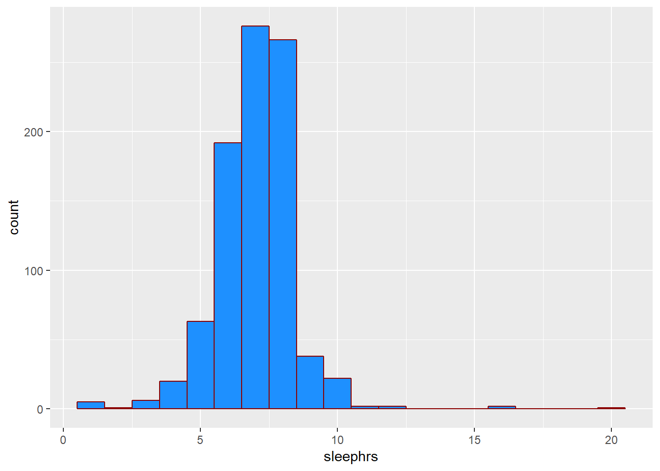

2.5.3 What’s the distribution of BMI?

ggplot(smartcle2, aes(bmi)) +
    geom_histogram(bins = 30, col = "white")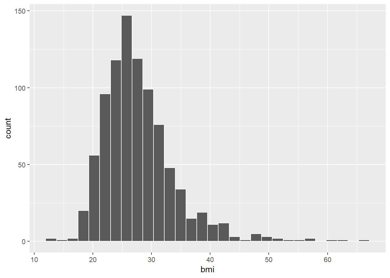

2.5.4 How many of the respondents have a BMI below 30?

smartcle2 %>% count(bmi < 30) %>% mutate(proportion = n / sum(n))

# A tibble: 2 x 3
  `bmi < 30`     n proportion
  <lgl>      <int>      <dbl>
1 FALSE        253      0.282
2 TRUE         643      0.718

2.5.5 How many of the respondents who have a BMI < 30 exercised?

smartcle2 %>% count(exerany, bmi < 30) %>%
    group_by(exerany) %>%
    mutate(percent = 100*n/sum(n))

# A tibble: 4 x 4
# Groups:   exerany [2]
  exerany `bmi < 30`     n percent
    <int> <lgl>      <int>   <dbl>
1       0 FALSE         88    42.1
2       0 TRUE         121    57.9
3       1 FALSE        165    24.0
4       1 TRUE         522    76.0

2.5.6 Is obesity associated with sex, in these data?

smartcle2 %>% count(female, bmi < 30) %>%
    group_by(female) %>%
    mutate(percent = 100*n/sum(n))

# A tibble: 4 x 4
# Groups:   female [2]
  female `bmi < 30`     n percent
   <int> <lgl>      <int>   <dbl>
1      0 FALSE        105    28.2
2      0 TRUE         267    71.8
3      1 FALSE        148    28.2
4      1 TRUE         376    71.8

2.5.7 Comparing sleephrs summaries by obesity status

Can we compare the sleephrs means, medians and 75^th percentiles for respondents whose BMI is below 30 to the respondents whose BMI is not?

smartcle2 %>%
    group_by(bmi < 30) %>%
    summarize(mean(sleephrs), median(sleephrs), 
              q75 = quantile(sleephrs, 0.75))

# A tibble: 2 x 4
  `bmi < 30` `mean(sleephrs)` `median(sleephrs)`   q75
  <lgl>                 <dbl>              <int> <dbl>
1 FALSE                  6.93                  7     8
2 TRUE                   7.06                  7     8

2.5.8 The skim function within a pipe

The skim function works within pipes and with the other tidyverse functions.

smartcle2 %>%
    group_by(exerany) %>%
    skim(bmi, sleephrs)

Skim summary statistics
 n obs: 896 
 n variables: 10 
 group variables: exerany 

-- Variable type:integer ----------------------------------------------------------
 exerany variable missing complete   n mean   sd p0 p25 p50 p75 p100
       0 sleephrs       0      209 209 7    1.85  1   6   7   8   20
       1 sleephrs       0      687 687 7.03 1.34  1   6   7   8   16

-- Variable type:numeric ----------------------------------------------------------
 exerany variable missing complete   n  mean   sd    p0   p25   p50   p75
       0      bmi       0      209 209 29.57 7.46 18    24.11 28.49 33.13
       1      bmi       0      687 687 27.35 5.84 12.71 23.7  26.52 29.81
  p100
 66.06
 60.95

2.6 First Modeling Attempt: Can bmi predict physhealth?

We’ll start with an effort to predict physhealth using bmi. A natural graph would be a scatterplot.

ggplot(data = smartcle2, aes(x = bmi, y = physhealth)) +
    geom_point()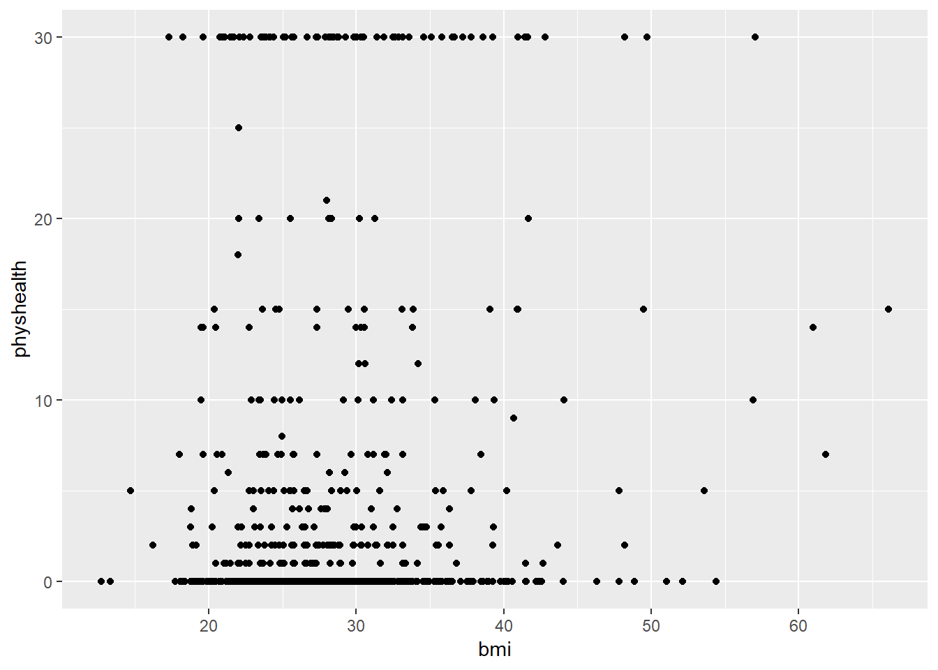

A good question to ask ourselves here might be: “In what BMI range can we make a reasonable prediction of physhealth?”

Now, we might take the plot above and add a simple linear model …

ggplot(data = smartcle2, aes(x = bmi, y = physhealth)) +
    geom_point() +
    geom_smooth(method = "lm", se = FALSE)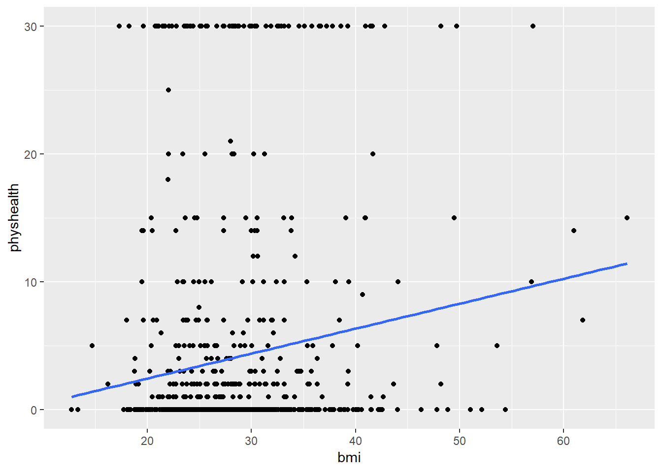

which shows the same least squares regression model that we can fit with the lm command.

2.6.1 Fitting a Simple Regression Model

model_A <- lm(physhealth ~ bmi, data = smartcle2)

model_A

Call:
lm(formula = physhealth ~ bmi, data = smartcle2)

Coefficients:
(Intercept)          bmi  
    -1.4514       0.1953  

summary(model_A)

Call:
lm(formula = physhealth ~ bmi, data = smartcle2)

Residuals:
   Min     1Q Median     3Q    Max 
-9.171 -4.057 -3.193 -1.576 28.073 

Coefficients:
            Estimate Std. Error t value Pr(>|t|)    
(Intercept) -1.45143    1.29185  -1.124    0.262    
bmi          0.19527    0.04521   4.319 1.74e-05 ***
---
Signif. codes:  0 '***' 0.001 '**' 0.01 '*' 0.05 '.' 0.1 ' ' 1

Residual standard error: 8.556 on 894 degrees of freedom
Multiple R-squared:  0.02044,   Adjusted R-squared:  0.01934 
F-statistic: 18.65 on 1 and 894 DF,  p-value: 1.742e-05

confint(model_A, level = 0.95)

                 2.5 %    97.5 %
(Intercept) -3.9868457 1.0839862
bmi          0.1065409 0.2840068

The model coefficients can be obtained by printing the model object, and the summary function provides several useful descriptions of the model’s residuals, its statistical significance, and quality of fit.

2.6.2 Model Summary for a Simple (One-Predictor) Regression

The fitted model predicts physhealth with the equation -1.45 + 0.195*bmi, as we can read off from the model coefficients.

Each of the 896 respondents included in the smartcle2 data makes a contribution to this model.

2.6.2.1 Residuals

Suppose Harry is one of the people in that group, and Harry’s data is bmi = 20, and physhealth = 3.

• Harry’s observed value of physhealth is just the value we have in the data for them, in this case, observed physhealth = 3 for Harry.
• Harry’s fitted or predicted physhealth value is the result of calculating -1.45 + 0.195*bmi for Harry. So, if Harry’s BMI was 20, then Harry’s predicted physhealth value is -1.45 + (0.195)(20) = 2.45.
• The residual for Harry is then his observed outcome minus his fitted outcome, so Harry has a residual of 3 - 2.45 = 0.55.
• Graphically, a residual represents vertical distance between the observed point and the fitted regression line.
• Points above the regression line will have positive residuals, and points below the regression line will have negative residuals. Points on the line have zero residuals.

The residuals are summarized at the top of the summary output for linear model.

• The mean residual will always be zero in an ordinary least squares model, but a five number summary of the residuals is provided by the summary, as is an estimated standard deviation of the residuals (called here the Residual standard error.)
• In the smartcle2 data, the minimum residual was -9.17, so for one subject, the observed value was 9.17 days smaller than the predicted value. This means that the prediction was 9.17 days too large for that subject.
• Similarly, the maximum residual was 28.07 days, so for one subject the prediction was 28.07 days too small. Not a strong performance.
• In a least squares model, the residuals are assumed to follow a Normal distribution, with mean zero, and standard deviation (for the smartcle2 data) of about 8.6 days. Thus, by the definition of a Normal distribution, we’d expect
• about 68% of the residuals to be between -8.6 and +8.6 days,
• about 95% of the residuals to be between -17.2 and +17.2 days,
• about all (99.7%) of the residuals to be between -25.8 and +25.8 days.

2.6.2.2 Coefficients section

The summary for a linear model shows Estimates, Standard Errors, t values and p values for each coefficient fit.

• The Estimates are the point estimates of the intercept and slope of bmi in our model.
• In this case, our estimated slope is 0.195, which implies that if Harry’s BMI is 20 and Sally’s BMI is 21, we predict that Sally’s physhealth will be 0.195 days larger than Harry’s.
• The Standard Errors are also provided for each estimate. We can create rough 95% confidence intervals by adding and subtracting two standard errors from each coefficient, or we can get a slightly more accurate answer with the confint function.
• Here, the 95% confidence interval for the slope of bmi is estimated to be (0.11, 0.28). This is a good measure of the uncertainty in the slope that is captured by our model. We are 95% confident in the process of building this interval, but this doesn’t mean we’re 95% sure that the true slope is actually in that interval.

Also available are a t value (just the Estimate divided by the Standard Error) and the appropriate p value for testing the null hypothesis that the true value of the coefficient is 0 against a two-tailed alternative.

• If a slope coefficient is statistically significantly different from 0, this implies that 0 will not be part of the uncertainty interval obtained through confint.
• If the slope was zero, it would suggest that bmi would add no predictive value to the model. But that’s unlikely here.

If the bmi slope coefficient is associated with a small p value, as in the case of our model_A, it suggests that the model including bmi is statistically significantly better at predicting physhealth than the model without bmi.

• Without bmi our model_A would become an intercept-only model, in this case, which would predict the mean physhealth for everyone, regardless of any other information.

2.6.2.3 Model Fit Summaries

The summary of a linear model also displays:

• The residual standard error and associated degrees of freedom for the residuals.
• For a simple (one-predictor) least regression like this, the residual degrees of freedom will be the sample size minus 2.
• The multiple R-squared (or coefficient of determination)
• This is interpreted as the proportion of variation in the outcome (physhealth) accounted for by the model, and will always fall between 0 and 1 as a result.
• Our model_A accounts for a mere 2% of the variation in physhealth.
• The Adjusted R-squared value “adjusts” for the size of our model in terms of the number of coefficients included in the model.
• The adjusted R-squared will always be less than the Multiple R-squared.
• We still hope to find models with relatively large adjusted R² values.
• In particular, we hope to find models where the adjusted R² isn’t substantially less than the Multiple R-squared.
• The adjusted R-squared is usually a better estimate of likely performance of our model in new data than is the Multiple R-squared.
• The adjusted R-squared result is no longer interpretable as a proportion of anything - in fact, it can fall below 0.
• We can obtain the adjusted R² from the raw R², the number of observations N and the number of predictors p included in the model, as follows:

\[ R^2_{adj} = 1 - \frac{(1 - R^2)(N - 1)}{N - p - 1}, \]

• The F statistic and p value from a global ANOVA test of the model.
  • Obtaining a statistically significant result here is usually pretty straightforward, since the comparison is between our model, and a model which simply predicts the mean value of the outcome for everyone.
  • In a simple (one-predictor) linear regression like this, the t statistic for the slope is just the square root of the F statistic, and the resulting p values for the slope’s t test and for the global F test will be identical.
• To see the complete ANOVA F test for this model, we can run anova(model_A).

anova(model_A)

Analysis of Variance Table

Response: physhealth
           Df Sum Sq Mean Sq F value    Pr(>F)    
bmi         1   1366  1365.5  18.655 1.742e-05 ***
Residuals 894  65441    73.2                      
---
Signif. codes:  0 '***' 0.001 '**' 0.01 '*' 0.05 '.' 0.1 ' ' 1

2.6.3 Using the broom package

The broom package has three functions of particular use in a linear regression model:

2.6.3.1 The tidy function

tidy builds a data frame/tibble containing information about the coefficients in the model, their standard errors, t statistics and p values.

tidy(model_A)

# A tibble: 2 x 5
  term        estimate std.error statistic   p.value
  <chr>          <dbl>     <dbl>     <dbl>     <dbl>
1 (Intercept)   -1.45     1.29       -1.12 0.262    
2 bmi            0.195    0.0452      4.32 0.0000174

2.6.3.2 The glance function

glance` builds a data frame/tibble containing summary statistics about the model, including

• the (raw) multiple R² and adjusted R^2
• sigma which is the residual standard error
• the F statistic, p.value model df and df.residual associated with the global ANOVA test, plus
• several statistics that will be useful in comparing models down the line:
• the model’s log likelihood function value, logLik
• the model’s Akaike’s Information Criterion value, AIC
• the model’s Bayesian Information Criterion value, BIC
• and the model’s deviance statistic

glance(model_A)

# A tibble: 1 x 11
  r.squared adj.r.squared sigma statistic p.value    df logLik   AIC   BIC
      <dbl>         <dbl> <dbl>     <dbl>   <dbl> <int>  <dbl> <dbl> <dbl>
1    0.0204        0.0193  8.56      18.7 1.74e-5     2 -3194. 6393. 6408.
# ... with 2 more variables: deviance <dbl>, df.residual <int>

2.6.3.3 The augment function

augment builds a data frame/tibble which adds fitted values, residuals and other diagnostic summaries that describe each observation to the original data used to fit the model, and this includes

• .fitted and .resid, the fitted and residual values, in addition to
• .hat, the leverage value for this observation
• .cooksd, the Cook’s distance measure of influence for this observation
• .stdresid, the standardized residual (think of this as a z-score - a measure of the residual divided by its associated standard deviation .sigma)
• and se.fit which will help us generate prediction intervals for the model downstream

Note that each of the new columns begins with . to avoid overwriting any data.

head(augment(model_A))

# A tibble: 6 x 9
  physhealth   bmi .fitted .se.fit  .resid    .hat .sigma .cooksd
       <int> <dbl>   <dbl>   <dbl>   <dbl>   <dbl>  <dbl>   <dbl>
1          0  26.7    3.76   0.291 -3.76   0.00115   8.56 1.12e-4
2          0  23.7    3.18   0.342 -3.18   0.00160   8.56 1.11e-4
3          1  26.9    3.81   0.289 -2.81   0.00114   8.56 6.15e-5
4          0  21.7    2.78   0.401 -2.78   0.00219   8.56 1.16e-4
5          5  24.1    3.25   0.333  1.75   0.00151   8.56 3.17e-5
6          4  27.6    3.95   0.286  0.0541 0.00112   8.56 2.24e-8
# ... with 1 more variable: .std.resid <dbl>

For more on the broom package, you may want to look at this vignette.

2.6.4 How does the model do? (Residuals vs. Fitted Values)

• Remember that the R² value was about 2%.

plot(model_A, which = 1)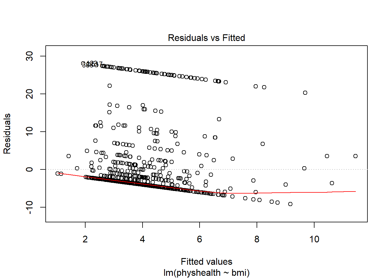

This is a plot of residuals vs. fitted values. The goal here is for this plot to look like a random scatter of points, perhaps like a “fuzzy football”, and that’s not what we have. Why?

If you prefer, here’s a ggplot2 version of a similar plot, now looking at standardized residuals instead of raw residuals, and adding a loess smooth and a linear fit to the result.

ggplot(augment(model_A), aes(x = .fitted, y = .std.resid)) +
    geom_point() +
    geom_smooth(method = "lm", se = FALSE, col = "red", linetype = "dashed") +
    geom_smooth(method = "loess", se = FALSE, col = "navy") +
    theme_bw()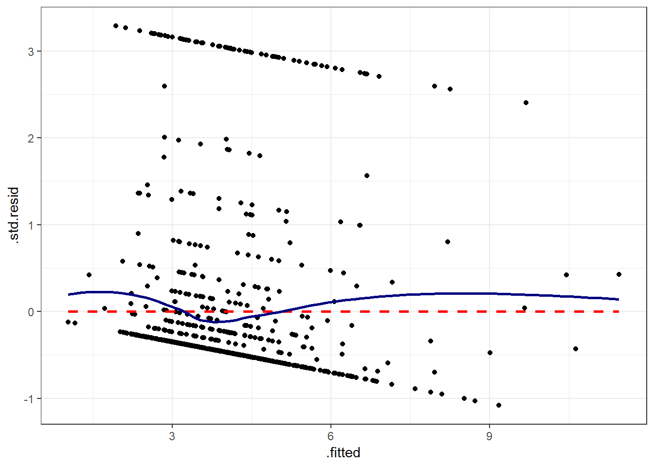

The problem we’re having here becomes, I think, a little more obvious if we look at what we’re predicting. Does physhealth look like a good candidate for a linear model?

ggplot(smartcle2, aes(x = physhealth)) +
geom_histogram(bins = 30, fill = "dodgerblue", color = "royalblue")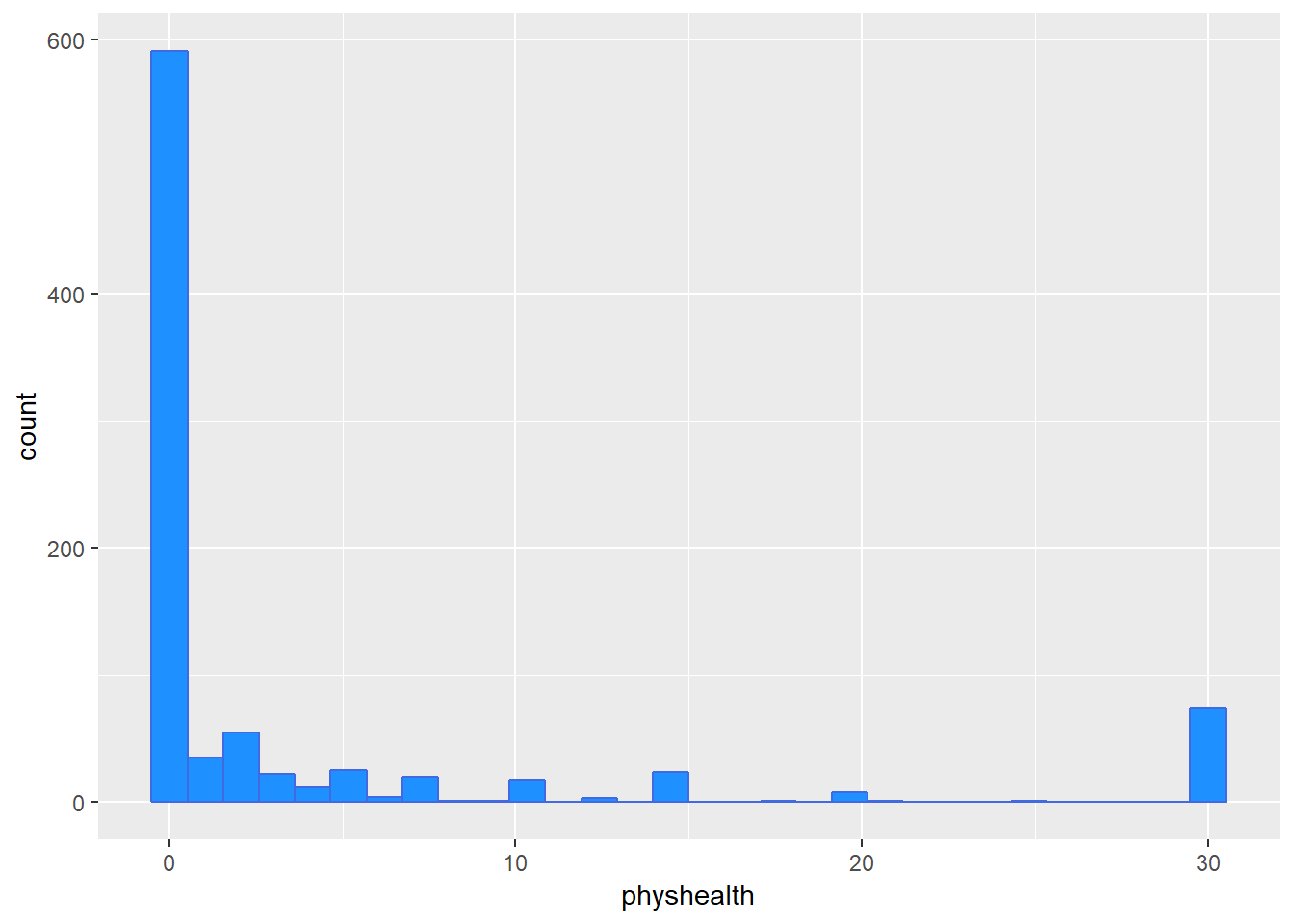

smartcle2 %>% count(physhealth == 0, physhealth == 30)

# A tibble: 3 x 3
  `physhealth == 0` `physhealth == 30`     n
  <lgl>             <lgl>              <int>
1 FALSE             FALSE                231
2 FALSE             TRUE                  74
3 TRUE              FALSE                591

No matter what model we fit, if we are predicting physhealth, and most of the data are values of 0 and 30, we have limited variation in our outcome, and so our linear model will be somewhat questionable just on that basis.

A normal Q-Q plot of the standardized residuals for our model_A shows this problem, too.

plot(model_A, which = 2)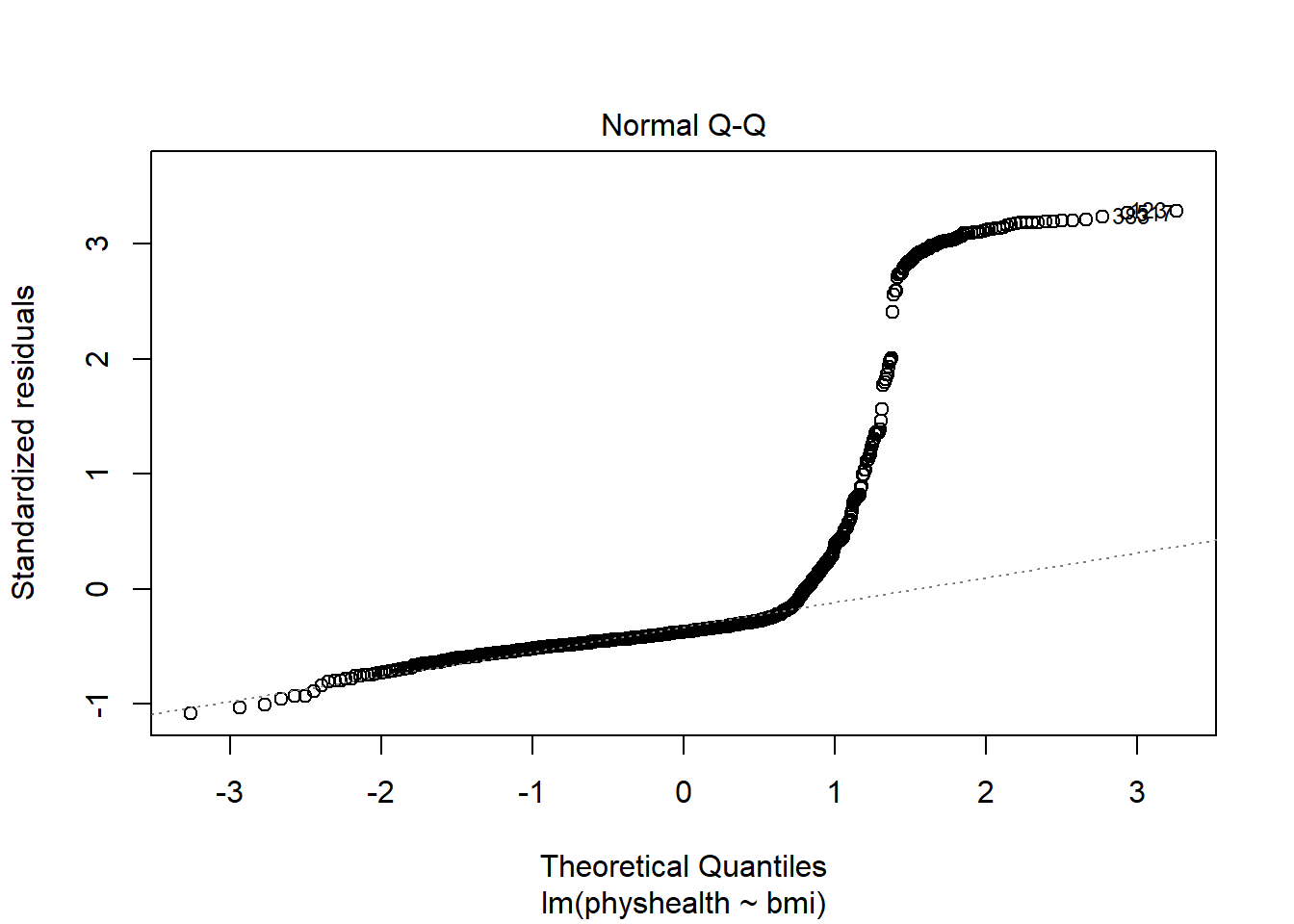

We’re going to need a method to deal with this sort of outcome, that has both a floor and a ceiling. We’ll get there eventually, but linear regression alone doesn’t look promising.

All right, so that didn’t go anywhere great. Let’s try again, with a new outcome.

2.7 A New Small Study: Predicting BMI

We’ll begin by investigating the problem of predicting bmi, at first with just three regression inputs: sex, exerany and sleephrs, in our new smartcle2 data set.

• The outcome of interest is bmi.
• Inputs to the regression model are:
  • female = 1 if the subject is female, and 0 if they are male
  • exerany = 1 if the subject exercised in the past 30 days, and 0 if they didn’t
  • sleephrs = hours slept in a typical 24-hour period (treated as quantitative)

2.7.1 Does female predict bmi well?

2.7.1.1 Graphical Assessment

ggplot(smartcle2, aes(x = female, y = bmi)) +
    geom_point()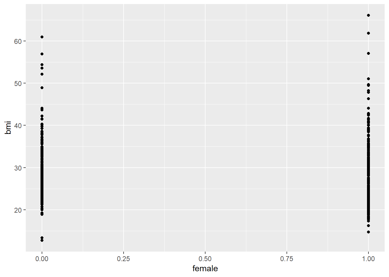

Not so helpful. We should probably specify that female is a factor, and try another plotting approach.

ggplot(smartcle2, aes(x = factor(female), y = bmi)) +
    geom_boxplot()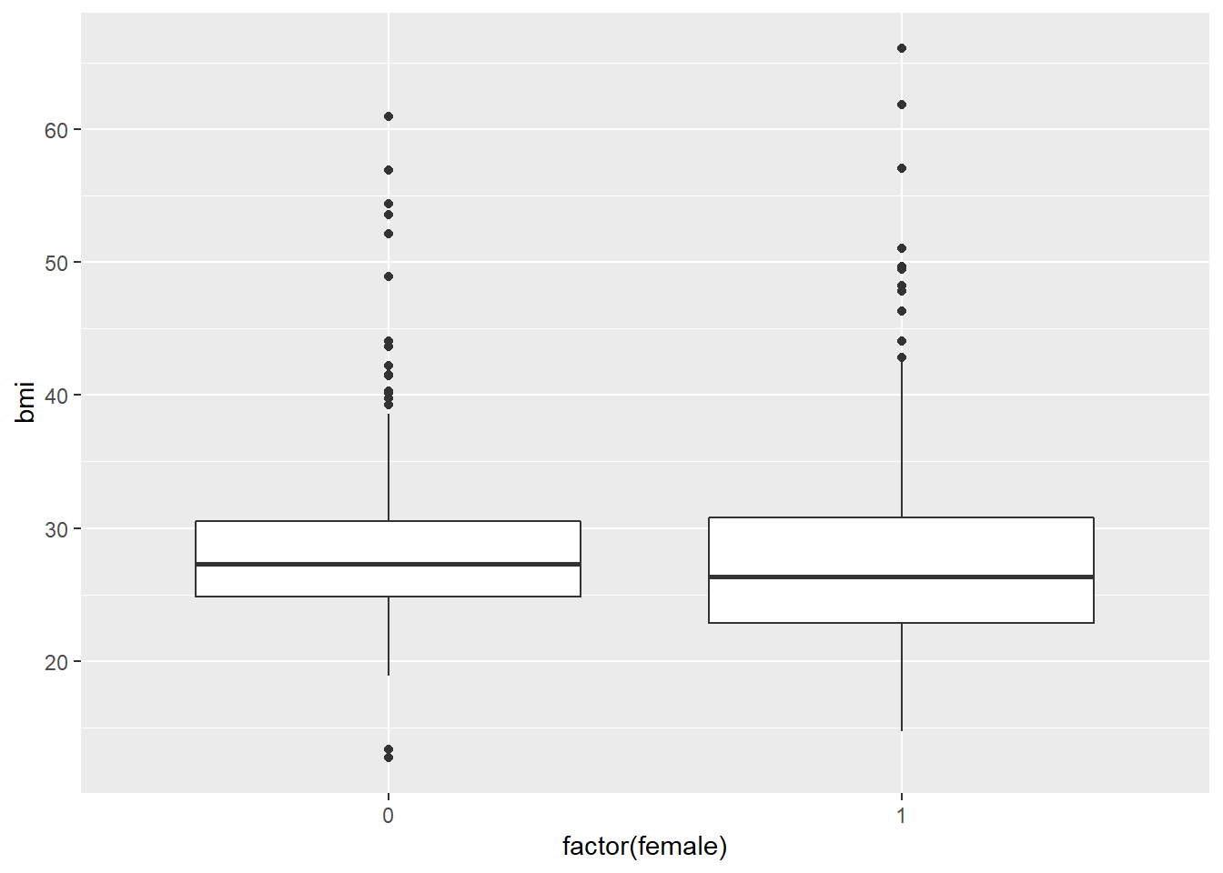

The median BMI looks a little higher for males. Let’s see if a model reflects that.

2.8 c2_m1: A simple t-test model

c2_m1 <- lm(bmi ~ female, data = smartcle2)
c2_m1

Call:
lm(formula = bmi ~ female, data = smartcle2)

Coefficients:
(Intercept)       female  
    28.3600      -0.8457  

summary(c2_m1)

Call:
lm(formula = bmi ~ female, data = smartcle2)

Residuals:
    Min      1Q  Median      3Q     Max 
-15.650  -4.129  -1.080   2.727  38.546 

Coefficients:
            Estimate Std. Error t value Pr(>|t|)    
(Intercept)  28.3600     0.3274  86.613   <2e-16 ***
female       -0.8457     0.4282  -1.975   0.0485 *  
---
Signif. codes:  0 '***' 0.001 '**' 0.01 '*' 0.05 '.' 0.1 ' ' 1

Residual standard error: 6.315 on 894 degrees of freedom
Multiple R-squared:  0.004345,  Adjusted R-squared:  0.003231 
F-statistic: 3.902 on 1 and 894 DF,  p-value: 0.04855

confint(c2_m1)

                2.5 %      97.5 %
(Intercept) 27.717372 29.00262801
female      -1.686052 -0.00539878

The model suggests, based on these 896 subjects, that

• our best prediction for males is BMI = 28.36 kg/m², and
• our best prediction for females is BMI = 28.36 - 0.85 = 27.51 kg/m².
• the mean difference between females and males is -0.85 kg/m² in BMI
• a 95% confidence (uncertainty) interval for that mean female - male difference in BMI ranges from -1.69 to -0.01
• the model accounts for 0.4% of the variation in BMI, so that knowing the respondent’s sex does very little to reduce the size of the prediction errors as compared to an intercept only model that would predict the overall mean (regardless of sex) for all subjects.
• the model makes some enormous errors, with one subject being predicted to have a BMI 38 points lower than his/her actual BMI.

Note that this simple regression model just gives us the t-test.

t.test(bmi ~ female, var.equal = TRUE, data = smartcle2)

    Two Sample t-test

data:  bmi by female
t = 1.9752, df = 894, p-value = 0.04855
alternative hypothesis: true difference in means is not equal to 0
95 percent confidence interval:
 0.00539878 1.68605160
sample estimates:
mean in group 0 mean in group 1 
       28.36000        27.51427 

2.9 c2_m2: Adding another predictor (two-way ANOVA without interaction)

When we add in the information about exerany to our original model, we might first picture the data. We could look at separate histograms,

ggplot(smartcle2, aes(x = bmi)) +
    geom_histogram(bins = 30) +
    facet_grid(female ~ exerany, labeller = label_both)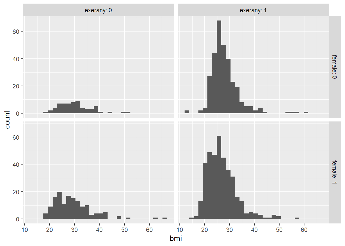

or maybe boxplots?

ggplot(smartcle2, aes(x = factor(female), y = bmi)) +
    geom_boxplot() +
    facet_wrap(~ exerany, labeller = label_both)

ggplot(smartcle2, aes(x = female, y = bmi))+
    geom_point(size = 3, alpha = 0.2) +
    theme_bw() +
    facet_wrap(~ exerany, labeller = label_both)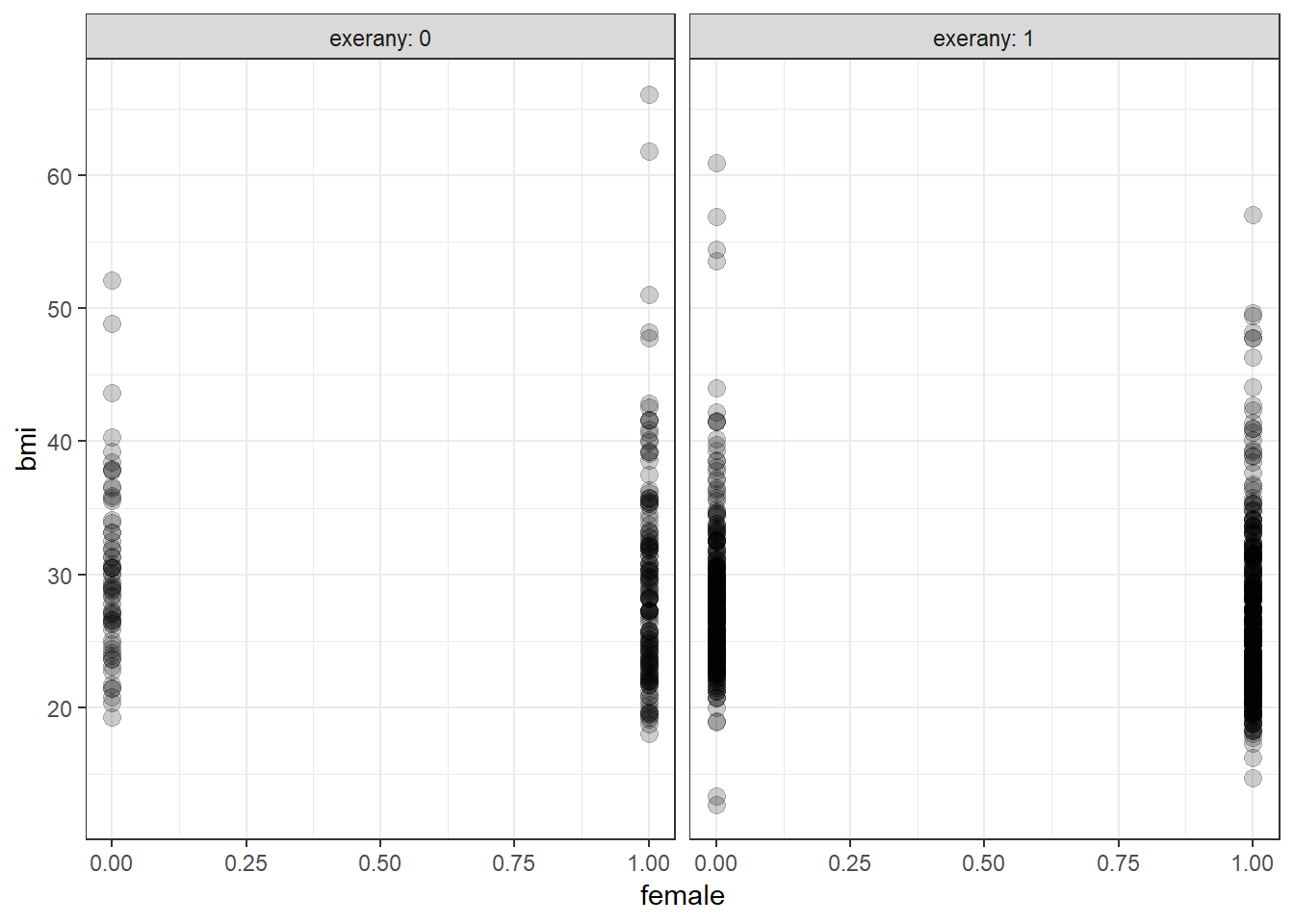

OK. Let’s try fitting a model.

c2_m2 <- lm(bmi ~ female + exerany, data = smartcle2)
c2_m2

Call:
lm(formula = bmi ~ female + exerany, data = smartcle2)

Coefficients:
(Intercept)       female      exerany  
     30.334       -1.095       -2.384  

This new model predicts only four predicted values:

• bmi = 30.334 if the subject is male and did not exercise (so female = 0 and exerany = 0)
• bmi = 30.334 - 1.095 = 29.239 if the subject is female and did not exercise (female = 1 and exerany = 0)
• bmi = 30.334 - 2.384 = 27.950 if the subject is male and exercised (so female = 0 and exerany = 1), and, finally
• bmi = 30.334 - 1.095 - 2.384 = 26.855 if the subject is female and exercised (so both female and exerany = 1).

For those who did not exercise, the model is:

• bmi = 30.334 - 1.095 female

and for those who did exercise, the model is:

• bmi = 27.95 - 1.095 female

Only the intercept of the bmi-female model changes depending on exerany.

summary(c2_m2)

Call:
lm(formula = bmi ~ female + exerany, data = smartcle2)

Residuals:
    Min      1Q  Median      3Q     Max 
-15.240  -4.091  -1.095   2.602  36.822 

Coefficients:
            Estimate Std. Error t value Pr(>|t|)    
(Intercept)  30.3335     0.5231   57.99  < 2e-16 ***
female       -1.0952     0.4262   -2.57   0.0103 *  
exerany      -2.3836     0.4965   -4.80 1.86e-06 ***
---
Signif. codes:  0 '***' 0.001 '**' 0.01 '*' 0.05 '.' 0.1 ' ' 1

Residual standard error: 6.239 on 893 degrees of freedom
Multiple R-squared:  0.02939,   Adjusted R-squared:  0.02722 
F-statistic: 13.52 on 2 and 893 DF,  p-value: 1.641e-06

confint(c2_m2)

                2.5 %     97.5 %
(Intercept) 29.306846 31.3602182
female      -1.931629 -0.2588299
exerany     -3.358156 -1.4090777

The slopes of both female and exerany have confidence intervals that are completely below zero, indicating that both female sex and exerany appear to be associated with reductions in bmi.

The R² value suggests that just under 3% of the variation in bmi is accounted for by this ANOVA model.

In fact, this regression (on two binary indicator variables) is simply a two-way ANOVA model without an interaction term.

anova(c2_m2)

Analysis of Variance Table

Response: bmi
           Df Sum Sq Mean Sq F value    Pr(>F)    
female      1    156  155.61  3.9977   0.04586 *  
exerany     1    897  896.93 23.0435 1.856e-06 ***
Residuals 893  34759   38.92                      
---
Signif. codes:  0 '***' 0.001 '**' 0.01 '*' 0.05 '.' 0.1 ' ' 1

2.10 c2_m3: Adding the interaction term (Two-way ANOVA with interaction)

Suppose we want to let the effect of female vary depending on the exerany status. Then we need to incorporate an interaction term in our model.

c2_m3 <- lm(bmi ~ female * exerany, data = smartcle2)
c2_m3

Call:
lm(formula = bmi ~ female * exerany, data = smartcle2)

Coefficients:
   (Intercept)          female         exerany  female:exerany  
       30.1359         -0.8104         -2.1450         -0.3592  

So, for example, for a male who exercises, this model predicts

• bmi = 30.136 - 0.810 (0) - 2.145 (1) - 0.359 (0)(1) = 30.136 - 2.145 = 27.991

And for a female who exercises, the model predicts

• bmi = 30.136 - 0.810 (1) - 2.145 (1) - 0.359 (1)(1) = 30.136 - 0.810 - 2.145 - 0.359 = 26.822

For those who did not exercise, the model is:

• bmi = 30.136 - 0.81 female

But for those who did exercise, the model is:

• bmi = (30.136 - 2.145) + (-0.810 + (-0.359)) female, or ,,,
• bmi = 27.991 - 1.169 female

Now, both the slope and the intercept of the bmi-female model change depending on exerany.

summary(c2_m3)

Call:
lm(formula = bmi ~ female * exerany, data = smartcle2)

Residuals:
    Min      1Q  Median      3Q     Max 
-15.281  -4.101  -1.061   2.566  36.734 

Coefficients:
               Estimate Std. Error t value Pr(>|t|)    
(Intercept)     30.1359     0.7802  38.624   <2e-16 ***
female          -0.8104     0.9367  -0.865   0.3872    
exerany         -2.1450     0.8575  -2.501   0.0125 *  
female:exerany  -0.3592     1.0520  -0.341   0.7328    
---
Signif. codes:  0 '***' 0.001 '**' 0.01 '*' 0.05 '.' 0.1 ' ' 1

Residual standard error: 6.242 on 892 degrees of freedom
Multiple R-squared:  0.02952,   Adjusted R-squared:  0.02625 
F-statistic: 9.044 on 3 and 892 DF,  p-value: 6.669e-06

confint(c2_m3)

                   2.5 %     97.5 %
(Intercept)    28.604610 31.6672650
female         -2.648893  1.0280526
exerany        -3.827886 -0.4620407
female:exerany -2.423994  1.7055248

In fact, this regression (on two binary indicator variables and a product term) is simply a two-way ANOVA model with an interaction term.

anova(c2_m3)

Analysis of Variance Table

Response: bmi
                Df Sum Sq Mean Sq F value    Pr(>F)    
female           1    156  155.61  3.9938   0.04597 *  
exerany          1    897  896.93 23.0207 1.878e-06 ***
female:exerany   1      5    4.54  0.1166   0.73283    
Residuals      892  34754   38.96                      
---
Signif. codes:  0 '***' 0.001 '**' 0.01 '*' 0.05 '.' 0.1 ' ' 1

The interaction term doesn’t change very much here. Its uncertainty interval includes zero, and the overall model still accounts for just under 3% of the variation in bmi.

2.11 c2_m4: Using female and sleephrs in a model for bmi

ggplot(smartcle2, aes(x = sleephrs, y = bmi, color = factor(female))) +
    geom_point() + 
    guides(col = FALSE) +
    geom_smooth(method = "lm", se = FALSE) +
    facet_wrap(~ female, labeller = label_both)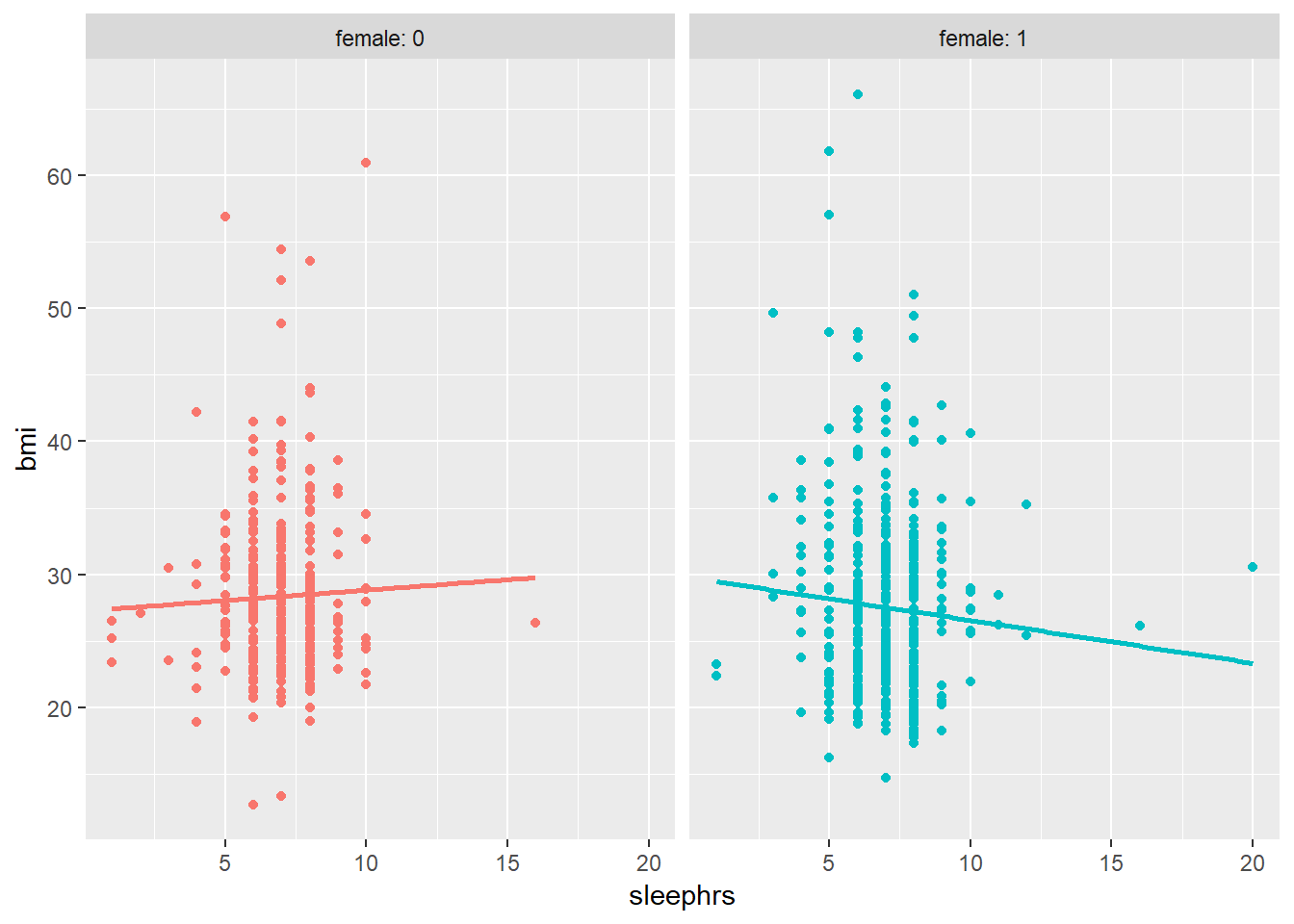 

Does the difference in slopes of bmi and sleephrs for males and females appear to be substantial and important?

c2_m4 <- lm(bmi ~ female * sleephrs, data = smartcle2)

summary(c2_m4)

Call:
lm(formula = bmi ~ female * sleephrs, data = smartcle2)

Residuals:
    Min      1Q  Median      3Q     Max 
-15.498  -4.179  -1.035   2.830  38.204 

Coefficients:
                Estimate Std. Error t value Pr(>|t|)    
(Intercept)      27.2661     1.6320  16.707   <2e-16 ***
female            2.5263     2.0975   1.204    0.229    
sleephrs          0.1569     0.2294   0.684    0.494    
female:sleephrs  -0.4797     0.2931  -1.636    0.102    
---
Signif. codes:  0 '***' 0.001 '**' 0.01 '*' 0.05 '.' 0.1 ' ' 1

Residual standard error: 6.31 on 892 degrees of freedom
Multiple R-squared:  0.008341,  Adjusted R-squared:  0.005006 
F-statistic: 2.501 on 3 and 892 DF,  p-value: 0.05818

Does it seem as though the addition of sleephrs has improved our model substantially over a model with female alone (which, you recall, was c2_m1)?

Since the c2_m4 model contains the c2_m1 model’s predictors as a subset and the outcome is the same for each model, we consider the models nested and have some extra tools available to compare them.

• I might start by looking at the basic summaries for each model.

glance(c2_m4)

# A tibble: 1 x 11
  r.squared adj.r.squared sigma statistic p.value    df logLik   AIC   BIC
      <dbl>         <dbl> <dbl>     <dbl>   <dbl> <int>  <dbl> <dbl> <dbl>
1   0.00834       0.00501  6.31      2.50  0.0582     4 -2920. 5850. 5874.
# ... with 2 more variables: deviance <dbl>, df.residual <int>

glance(c2_m1)

# A tibble: 1 x 11
  r.squared adj.r.squared sigma statistic p.value    df logLik   AIC   BIC
      <dbl>         <dbl> <dbl>     <dbl>   <dbl> <int>  <dbl> <dbl> <dbl>
1   0.00435       0.00323  6.32      3.90  0.0485     2 -2922. 5849. 5864.
# ... with 2 more variables: deviance <dbl>, df.residual <int>

• The R² is twice as large for the model with sleephrs, but still very tiny.
• The p value for the global ANOVA test is actually less significant in c2_m4 than in c2_m1.
• Smaller AIC and smaller BIC statistics are more desirable. Here, there’s little to choose from, but c2_m1 is a little better on each standard.
• We might also consider a significance test by looking at an ANOVA model comparison. This is only appropriate because c2_m1 is nested in c2_m4.

anova(c2_m4, c2_m1)

Analysis of Variance Table

Model 1: bmi ~ female * sleephrs
Model 2: bmi ~ female
  Res.Df   RSS Df Sum of Sq      F Pr(>F)
1    892 35512                           
2    894 35656 -2   -143.11 1.7973 0.1663

The addition of the sleephrs term picked up 143 in the sum of squares column, at a cost of two degrees of freedom, yielding a p value of 0.166, suggesting that this isn’t a significant improvement over the model that just did a t-test on female.

2.12 Making Predictions with a Linear Regression Model

Recall model 4, which yields predictions for body mass index on the basis of the main effects of sex (female) and hours of sleep (sleephrs) and their interaction.

c2_m4

Call:
lm(formula = bmi ~ female * sleephrs, data = smartcle2)

Coefficients:
    (Intercept)           female         sleephrs  female:sleephrs  
        27.2661           2.5263           0.1569          -0.4797  

2.12.1 Fitting an Individual Prediction and 95% Prediction Interval

What do we predict for the bmi of a subject who is female and gets 8 hours of sleep per night?

c2_new1 <- data_frame(female = 1, sleephrs = 8)
predict(c2_m4, newdata = c2_new1, interval = "prediction", level = 0.95)

       fit     lwr     upr
1 27.21065 14.8107 39.6106

The predicted bmi for this new subject is 27.61. The prediction interval shows the bounds of a 95% uncertainty interval for a predicted bmi for an individual female subject who gets 8 hours of sleep on average per evening. From the predict function applied to a linear model, we can get the prediction intervals for any new data points in this manner.

2.12.2 Confidence Interval for an Average Prediction

• What do we predict for the average body mass index of a population of subjects who are female and sleep for 8 hours?

predict(c2_m4, newdata = c2_new1, interval = "confidence", level = 0.95)

       fit      lwr      upr
1 27.21065 26.57328 27.84801

• How does this result compare to the prediction interval?

2.12.3 Fitting Multiple Individual Predictions to New Data

• How does our prediction change for a respondent if they instead get 7, or 9 hours of sleep? What if they are male, instead of female?

c2_new2 <- data_frame(subjectid = 1001:1006, female = c(1, 1, 1, 0, 0, 0), sleephrs = c(7, 8, 9, 7, 8, 9))
pred2 <- predict(c2_m4, newdata = c2_new2, interval = "prediction", level = 0.95) %>% tbl_df

result2 <- bind_cols(c2_new2, pred2)
result2

# A tibble: 6 x 6
  subjectid female sleephrs   fit   lwr   upr
      <int>  <dbl>    <dbl> <dbl> <dbl> <dbl>
1      1001      1        7  27.5  15.1  39.9
2      1002      1        8  27.2  14.8  39.6
3      1003      1        9  26.9  14.5  39.3
4      1004      0        7  28.4  16.0  40.8
5      1005      0        8  28.5  16.1  40.9
6      1006      0        9  28.7  16.2  41.1

The result2 tibble contains predictions for each scenario.

• Which has a bigger impact on these predictions and prediction intervals? A one category change in female or a one hour change in sleephrs?

2.12.4 Simulation to represent predictive uncertainty in Model 4

Suppose we want to predict the bmi of a female subject who sleeps for eight hours per night. As we have seen, we can do this automatically for a linear model like this one, using the predict function applied to the linear model, but a simulation prediction can also be done. Recall the detail of c2_m4:

c2_m4

Call:
lm(formula = bmi ~ female * sleephrs, data = smartcle2)

Coefficients:
    (Intercept)           female         sleephrs  female:sleephrs  
        27.2661           2.5263           0.1569          -0.4797  

glance(c2_m4)

# A tibble: 1 x 11
  r.squared adj.r.squared sigma statistic p.value    df logLik   AIC   BIC
      <dbl>         <dbl> <dbl>     <dbl>   <dbl> <int>  <dbl> <dbl> <dbl>
1   0.00834       0.00501  6.31      2.50  0.0582     4 -2920. 5850. 5874.
# ... with 2 more variables: deviance <dbl>, df.residual <int>

We see that the residual standard error for our bmi predictions with this model is 6.31.

For a female respondent sleeping eight hours, recall that our point estimate (predicted value) of bmi is 27.21

predict(c2_m4, newdata = c2_new1, interval = "prediction", level = 0.95)

       fit     lwr     upr
1 27.21065 14.8107 39.6106

The standard deviation is 6.31, so we could summarize the predictive distribution with a command that tells R to draw 1000 random numbers from a normal distribution with mean 27.21 and standard deviation 6.31. Let’s summarize that and get a quick picture.

set.seed(432094)
pred.sim <- rnorm(1000, 27.21, 6.31)
hist(pred.sim, col = "royalblue")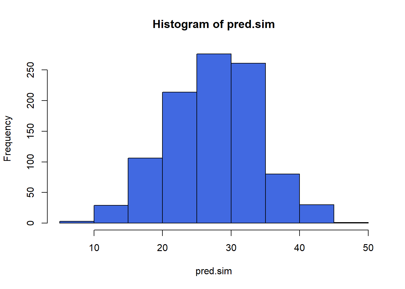

mean(pred.sim)

[1] 27.41856

quantile(pred.sim, c(0.025, 0.975))

    2.5%    97.5% 
14.48487 40.16778 

How do these results compare to the prediction interval of (14.81, 39.61) that we generated earlier?

2.13 Centering the model

Our model c2_m4 has four predictors (the constant, sleephrs, female and their interaction) but just two inputs (female and sleephrs.) If we center the quantitative input sleephrs before building the model, we get a more interpretable interaction term.

smartcle2_c <- smartcle2 %>%
    mutate(sleephrs_c = sleephrs - mean(sleephrs))

c2_m4_c <- lm(bmi ~ female * sleephrs_c, data = smartcle2_c)

summary(c2_m4_c)

Call:
lm(formula = bmi ~ female * sleephrs_c, data = smartcle2_c)

Residuals:
    Min      1Q  Median      3Q     Max 
-15.498  -4.179  -1.035   2.830  38.204 

Coefficients:
                  Estimate Std. Error t value Pr(>|t|)    
(Intercept)        28.3681     0.3274  86.658   <2e-16 ***
female             -0.8420     0.4280  -1.967   0.0495 *  
sleephrs_c          0.1569     0.2294   0.684   0.4940    
female:sleephrs_c  -0.4797     0.2931  -1.636   0.1021    
---
Signif. codes:  0 '***' 0.001 '**' 0.01 '*' 0.05 '.' 0.1 ' ' 1

Residual standard error: 6.31 on 892 degrees of freedom
Multiple R-squared:  0.008341,  Adjusted R-squared:  0.005006 
F-statistic: 2.501 on 3 and 892 DF,  p-value: 0.05818

What has changed as compared to the original c2_m4?

• Our original model was bmi = 27.26 + 2.53 female + 0.16 sleephrs - 0.48 female x sleephrs
• Our new model is bmi = 28.37 - 0.84 female + 0.16 centered sleephrs - 0.48 female x centered sleephrs.

So our new model on centered data is:

• 28.37 + 0.16 centered sleephrs_c for male subjects, and
• (28.37 - 0.84) + (0.16 - 0.48) centered sleephrs_c, or 27.53 - 0.32 centered sleephrs_c for female subjects.

In our new (centered sleephrs_c) model,

• the main effect of female now corresponds to a predictive difference (female - male) in bmi with sleephrs at its mean value, 7.02 hours,
• the intercept term is now the predicted bmi for a male respondent who sleeps an average number of hours, and
• the product term corresponds to the change in the slope of centered sleephrs_c on bmi for a female rather than a male subject, while
• the residual standard deviation and the R-squared values remain unchanged from the model before centering.

2.13.1 Plot of Model 4 on Centered sleephrs: c2_m4_c

ggplot(smartcle2_c, aes(x = sleephrs_c, y = bmi, group = female, col = factor(female))) +
    geom_point(alpha = 0.5, size = 2) +
    geom_smooth(method = "lm", se = FALSE) +
    guides(color = FALSE) +
    labs(x = "Sleep Hours, centered", y = "Body Mass Index",
         title = "Model `c2_m4` on centered data") +
    facet_wrap(~ female, labeller = label_both)

2.14 Rescaling an input by subtracting the mean and dividing by 2 standard deviations

Centering helped us interpret the main effects in the regression, but it still leaves a scaling problem.

• The female coefficient estimate is much larger than that of sleephrs, but this is misleading, considering that we are comparing the complete change in one variable (sex = female or not) to a 1-hour change in average sleep.
• Gelman and Hill (2007) recommend all continuous predictors be scaled by dividing by 2 standard deviations, so that:
  • a 1-unit change in the rescaled predictor corresponds to a change from 1 standard deviation below the mean, to 1 standard deviation above.
  • an unscaled binary (1/0) predictor with 50% probability of occurring will be exactly comparable to a rescaled continuous predictor done in this way.

smartcle2_rescale <- smartcle2 %>%
    mutate(sleephrs_z = (sleephrs - mean(sleephrs))/(2*sd(sleephrs)))

2.14.1 Refitting model c2_m4 to the rescaled data

c2_m4_z <- lm(bmi ~ female * sleephrs_z, data = smartcle2_rescale)

summary(c2_m4_z)

Call:
lm(formula = bmi ~ female * sleephrs_z, data = smartcle2_rescale)

Residuals:
    Min      1Q  Median      3Q     Max 
-15.498  -4.179  -1.035   2.830  38.204 

Coefficients:
                  Estimate Std. Error t value Pr(>|t|)    
(Intercept)        28.3681     0.3274  86.658   <2e-16 ***
female             -0.8420     0.4280  -1.967   0.0495 *  
sleephrs_z          0.4637     0.6778   0.684   0.4940    
female:sleephrs_z  -1.4173     0.8661  -1.636   0.1021    
---
Signif. codes:  0 '***' 0.001 '**' 0.01 '*' 0.05 '.' 0.1 ' ' 1

Residual standard error: 6.31 on 892 degrees of freedom
Multiple R-squared:  0.008341,  Adjusted R-squared:  0.005006 
F-statistic: 2.501 on 3 and 892 DF,  p-value: 0.05818

2.14.2 Interpreting the model on rescaled data

What has changed as compared to the original c2_m4?

• Our original model was bmi = 27.26 + 2.53 female + 0.16 sleephrs - 0.48 female x sleephrs
• Our model on centered sleephrs was bmi = 28.37 - 0.84 female + 0.16 centered sleephrs_c - 0.48 female x centered sleephrs_c.
• Our new model on rescaled sleephrs is bmi = 28.37 - 0.84 female + 0.46 rescaled sleephrs_z - 1.42 female x rescaled sleephrs_z.

So our rescaled model is:

• 28.37 + 0.46 rescaled sleephrs_z for male subjects, and
• (28.37 - 0.84) + (0.46 - 1.42) rescaled sleephrs_z, or 27.53 - 0.96 rescaled sleephrs_z for female subjects.

In this new rescaled (sleephrs_z) model, then,

• the main effect of female, -0.84, still corresponds to a predictive difference (female - male) in bmi with sleephrs at its mean value, 7.02 hours,
• the intercept term is still the predicted bmi for a male respondent who sleeps an average number of hours, and
• the residual standard deviation and the R-squared values remain unchanged,

as before, but now we also have that:

• the coefficient of sleephrs_z indicates the predictive difference in bmi associated with a change in sleephrs of 2 standard deviations (from one standard deviation below the mean of 7.02 to one standard deviation above 7.02.)
  • Since the standard deviation of sleephrs is 1.48, this corresponds to a change from 5.54 hours per night to 8.50 hours per night.
• the coefficient of the product term (-1.42) corresponds to the change in the coefficient of sleephrs_z for females as compared to males.

2.14.3 Plot of model on rescaled data

ggplot(smartcle2_rescale, aes(x = sleephrs_z, y = bmi, 
                              group = female, col = factor(female))) +
    geom_point(alpha = 0.5) +
    geom_smooth(method = "lm", size = 1.5) +
    scale_color_discrete(name = "Is subject female?") +
    labs(x = "Sleep Hours, standardized (2 sd)", y = "Body Mass Index",
         title = "Model `c2_m4_z` on rescaled data")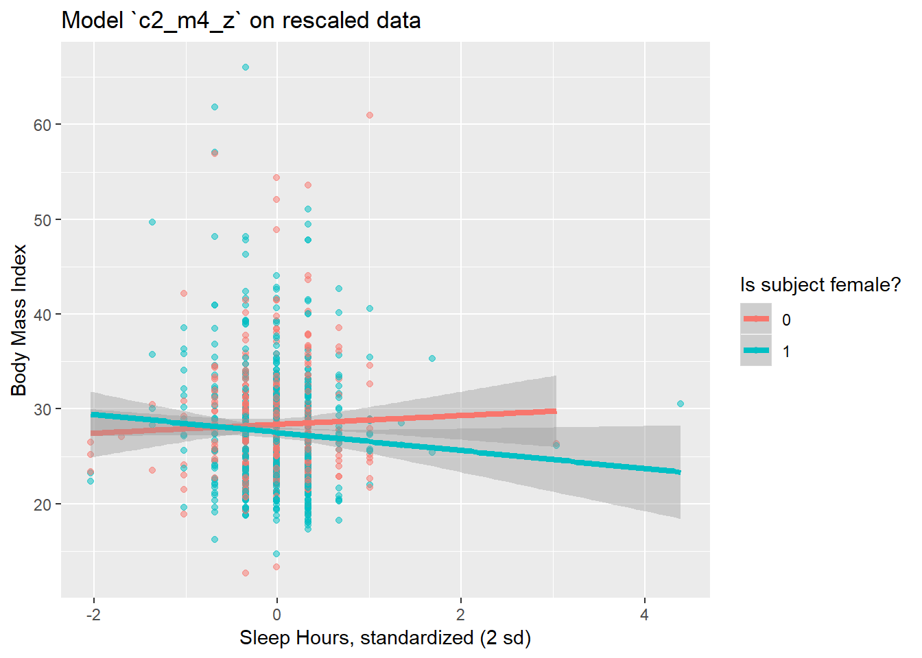

2.15 c2_m5: What if we add more variables?

We can boost our R² a bit, to over 5%, by adding in two new variables, related to whether or not the subject (in the past 30 days) used the internet, and on how many days the subject drank alcoholic beverages.

c2_m5 <- lm(bmi ~ female + exerany + sleephrs + internet30 + alcdays,
         data = smartcle2)
summary(c2_m5)

Call:
lm(formula = bmi ~ female + exerany + sleephrs + internet30 + 
    alcdays, data = smartcle2)

Residuals:
    Min      1Q  Median      3Q     Max 
-16.147  -3.997  -0.856   2.487  35.965 

Coefficients:
            Estimate Std. Error t value Pr(>|t|)    
(Intercept) 30.84066    1.18458  26.035  < 2e-16 ***
female      -1.28801    0.42805  -3.009   0.0027 ** 
exerany     -2.42161    0.49853  -4.858 1.40e-06 ***
sleephrs    -0.14118    0.13988  -1.009   0.3131    
internet30   1.38916    0.54252   2.561   0.0106 *  
alcdays     -0.10460    0.02595  -4.030 6.04e-05 ***
---
Signif. codes:  0 '***' 0.001 '**' 0.01 '*' 0.05 '.' 0.1 ' ' 1

Residual standard error: 6.174 on 890 degrees of freedom
Multiple R-squared:  0.05258,   Adjusted R-squared:  0.04726 
F-statistic: 9.879 on 5 and 890 DF,  p-value: 3.304e-09

1. Here’s the ANOVA for this model. What can we study with this?

anova(c2_m5)

Analysis of Variance Table

Response: bmi
            Df Sum Sq Mean Sq F value    Pr(>F)    
female       1    156  155.61  4.0818   0.04365 *  
exerany      1    897  896.93 23.5283 1.453e-06 ***
sleephrs     1     33   32.90  0.8631   0.35313    
internet30   1    178  178.33  4.6779   0.03082 *  
alcdays      1    619  619.26 16.2443 6.044e-05 ***
Residuals  890  33928   38.12                      
---
Signif. codes:  0 '***' 0.001 '**' 0.01 '*' 0.05 '.' 0.1 ' ' 1

2. Consider the revised output below. Now what can we study?

anova(lm(bmi ~ exerany + internet30 + alcdays + female + sleephrs,
         data = smartcle2))

Analysis of Variance Table

Response: bmi
            Df Sum Sq Mean Sq F value    Pr(>F)    
exerany      1    795  795.46 20.8664 5.618e-06 ***
internet30   1    212  211.95  5.5599 0.0185925 *  
alcdays      1    486  486.03 12.7496 0.0003752 ***
female       1    351  350.75  9.2010 0.0024891 ** 
sleephrs     1     39   38.83  1.0186 0.3131176    
Residuals  890  33928   38.12                      
---
Signif. codes:  0 '***' 0.001 '**' 0.01 '*' 0.05 '.' 0.1 ' ' 1

3. What does the output below let us conclude?

anova(lm(bmi ~ exerany + internet30 + alcdays + female + sleephrs, 
         data = smartcle2),
      lm(bmi ~ exerany + female + alcdays, 
         data = smartcle2))

Analysis of Variance Table

Model 1: bmi ~ exerany + internet30 + alcdays + female + sleephrs
Model 2: bmi ~ exerany + female + alcdays
  Res.Df   RSS Df Sum of Sq      F  Pr(>F)  
1    890 33928                              
2    892 34221 -2    -293.2 3.8456 0.02173 *
---
Signif. codes:  0 '***' 0.001 '**' 0.01 '*' 0.05 '.' 0.1 ' ' 1

4. What does it mean for the models to be “nested”?

2.16 c2_m6: Would adding self-reported health help?

And we can do even a bit better than that by adding in a multi-categorical measure: self-reported general health.

c2_m6 <- lm(bmi ~ female + exerany + sleephrs + internet30 + alcdays + genhealth,
         data = smartcle2)
summary(c2_m6)

Call:
lm(formula = bmi ~ female + exerany + sleephrs + internet30 + 
    alcdays + genhealth, data = smartcle2)

Residuals:
    Min      1Q  Median      3Q     Max 
-16.331  -3.813  -0.838   2.679  34.166 

Coefficients:
                    Estimate Std. Error t value Pr(>|t|)    
(Intercept)         26.49498    1.31121  20.206  < 2e-16 ***
female              -0.85520    0.41969  -2.038 0.041879 *  
exerany             -1.61968    0.50541  -3.205 0.001400 ** 
sleephrs            -0.12719    0.13613  -0.934 0.350368    
internet30           2.02498    0.53898   3.757 0.000183 ***
alcdays             -0.08431    0.02537  -3.324 0.000925 ***
genhealth2_VeryGood  2.10537    0.59408   3.544 0.000415 ***
genhealth3_Good      4.08245    0.60739   6.721 3.22e-11 ***
genhealth4_Fair      4.99213    0.80178   6.226 7.37e-10 ***
genhealth5_Poor      3.11025    1.12614   2.762 0.005866 ** 
---
Signif. codes:  0 '***' 0.001 '**' 0.01 '*' 0.05 '.' 0.1 ' ' 1

Residual standard error: 5.993 on 886 degrees of freedom
Multiple R-squared:  0.1115,    Adjusted R-squared:  0.1024 
F-statistic: 12.35 on 9 and 886 DF,  p-value: < 2.2e-16

1. If Harry and Marty have the same values of female, exerany, sleephrs, internet30 and alcdays, but Harry rates his health as Good, and Marty rates his as Fair, then what is the difference in the predictions? Who is predicted to have a larger BMI, and by how much?

2. What does this normal probability plot of the residuals suggest?

plot(c2_m6, which = 2)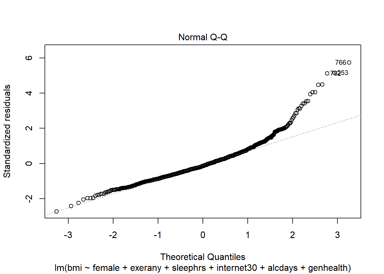

2.17 c2_m7: What if we added the menthealth variable?

c2_m7 <- lm(bmi ~ female + exerany + sleephrs + internet30 + alcdays + 
                genhealth + physhealth + menthealth,
         data = smartcle2)

summary(c2_m7)

Call:
lm(formula = bmi ~ female + exerany + sleephrs + internet30 + 
    alcdays + genhealth + physhealth + menthealth, data = smartcle2)

Residuals:
    Min      1Q  Median      3Q     Max 
-16.060  -3.804  -0.890   2.794  33.972 

Coefficients:
                    Estimate Std. Error t value Pr(>|t|)    
(Intercept)         25.88208    1.31854  19.629  < 2e-16 ***
female              -0.96435    0.41908  -2.301 0.021616 *  
exerany             -1.43171    0.50635  -2.828 0.004797 ** 
sleephrs            -0.08033    0.13624  -0.590 0.555583    
internet30           2.00267    0.53759   3.725 0.000207 ***
alcdays             -0.07997    0.02528  -3.163 0.001614 ** 
genhealth2_VeryGood  2.09533    0.59238   3.537 0.000425 ***
genhealth3_Good      3.90949    0.60788   6.431 2.07e-10 ***
genhealth4_Fair      4.27152    0.83986   5.086 4.47e-07 ***
genhealth5_Poor      1.26021    1.31556   0.958 0.338361    
physhealth           0.06088    0.03005   2.026 0.043064 *  
menthealth           0.06636    0.03177   2.089 0.037021 *  
---
Signif. codes:  0 '***' 0.001 '**' 0.01 '*' 0.05 '.' 0.1 ' ' 1

Residual standard error: 5.964 on 884 degrees of freedom
Multiple R-squared:  0.1219,    Adjusted R-squared:  0.111 
F-statistic: 11.16 on 11 and 884 DF,  p-value: < 2.2e-16

2.18 Key Regression Assumptions for Building Effective Prediction Models

1. Validity - the data you are analyzing should map to the research question you are trying to answer.
   • The outcome should accurately reflect the phenomenon of interest.
   • The model should include all relevant predictors. (It can be difficult to decide which predictors are necessary, and what to do with predictors that have large standard errors.)
   • The model should generalize to all of the cases to which it will be applied.
   • Can the available data answer our question reliably?
2. Additivity and linearity - most important assumption of a regression model is that its deterministic component is a linear function of the predictors. We often think about transformations in this setting.
3. Independence of errors - errors from the prediction line are independent of each other
4. Equal variance of errors - if this is violated, we can more efficiently estimate parameters using weighted least squares approaches, where each point is weighted inversely proportional to its variance, but this doesn’t affect the coefficients much, if at all.
5. Normality of errors - not generally important for estimating the regression line

2.18.1 Checking Assumptions in model c2_m7

1. How does the assumption of linearity behind this model look?

plot(c2_m7, which = 1)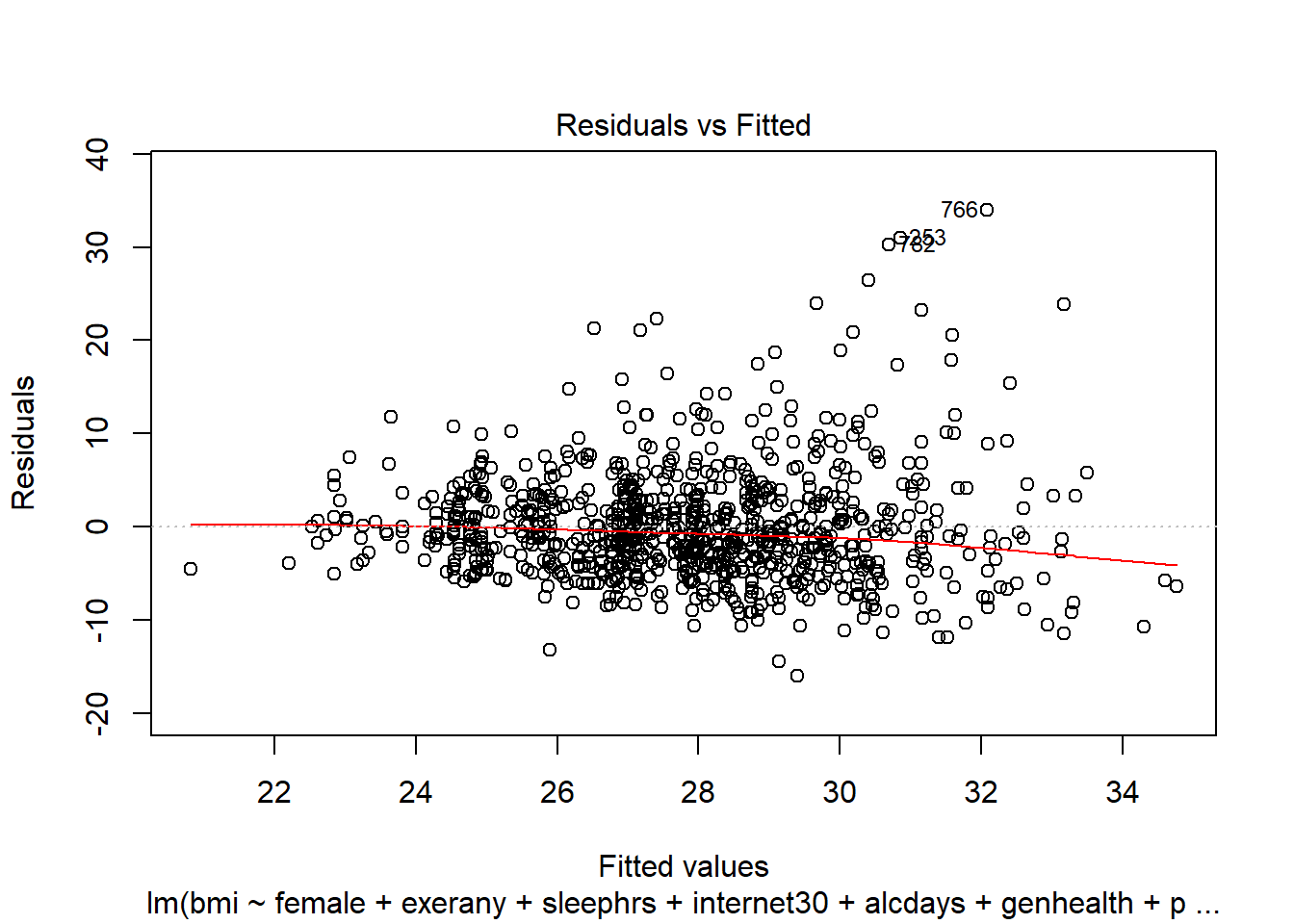

We see no strong signs of serious non-linearity here. There’s no obvious curve in the plot, for example.

2. What can we conclude from the plot below?

plot(c2_m7, which = 5)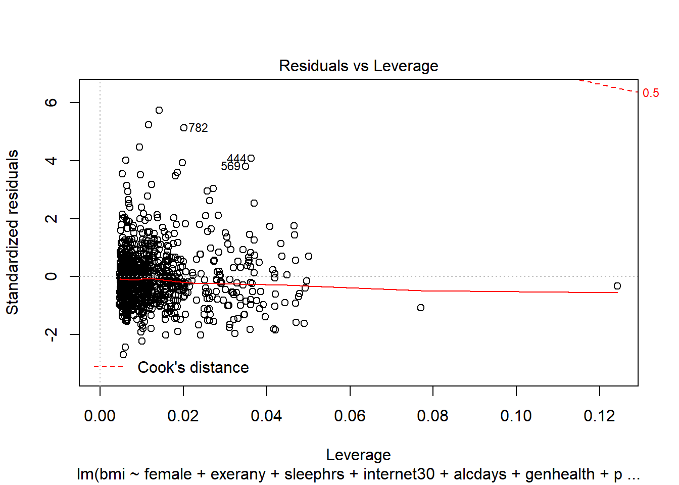

This plot can help us identify points with large standardized residuals, large leverage values, and large influence on the model (as indicated by large values of Cook’s distance.) In this case, I see no signs of any points used in the model with especially large influence, although there are some poorly fitted points (with especially large standardized residuals.)

References

Gelman, Andrew, and Jennifer Hill. 2007. Data Analysis Using Regression and Multilevel/Hierarchical Models. New York: Cambridge University Press.