Chapter 14 Logistic Regression and the smartcle1 data
14.1 The smartcle1 data
Recall that the smartcle1.csv data file available on the Data and Code page of our website describes information on 11 variables for 1036 respondents to the BRFSS 2016, who live in the Cleveland-Elyria, OH, Metropolitan Statistical Area. As we’ve discussed in previous work, the variables in the smartcle1.csv file are listed below, along with (in some cases) the BRFSS items that generate these responses.
| Variable | Description |
|---|---|
SEQNO |
respondent identification number (all begin with 2016) |
physhealth |
Now thinking about your physical health, which includes physical illness and injury, for how many days during the past 30 days was your physical health not good? |
menthealth |
Now thinking about your mental health, which includes stress, depression, and problems with emotions, for how many days during the past 30 days was your mental health not good? |
poorhealth |
During the past 30 days, for about how many days did poor physical or mental health keep you from doing your usual activities, such as self-care, work, or recreation? |
genhealth |
Would you say that in general, your health is … (five categories: Excellent, Very Good, Good, Fair or Poor) |
bmi |
Body mass index, in kg/m2 |
female |
Sex, 1 = female, 0 = male |
internet30 |
Have you used the internet in the past 30 days? (1 = yes, 0 = no) |
exerany |
During the past month, other than your regular job, did you participate in any physical activities or exercises such as running, calisthenics, golf, gardening, or walking for exercise? (1 = yes, 0 = no) |
sleephrs |
On average, how many hours of sleep do you get in a 24-hour period? |
alcdays |
How many days during the past 30 days did you have at least one drink of any alcoholic beverage such as beer, wine, a malt beverage or liquor? |
In this section, we’ll use some of the variables described above to predict the binary outcome: exerany.
14.2 Thinking About Non-Linear Terms
We have enough observations here to consider some non-linearity for our model.
In addition, since the genhealth variable is an ordinal variable and multi-categorical, we should consider how to model it. We have three options:
- include it as a factor in the model (the default approach)
- build a numeric version of that variable, and then restrict our model to treat that numeric variable as ordinal (forcing the categories to affect the
exeranyprobabilities in an ordinal way), rather than as a simple nominal factor (so that if the effect of fair vs. good was to decrease the probability of ‘exerany’, then the effect of poor vs. good would have to decrease the probability at least as much as fair vs. good did.) Treating thegenhealthvariable as ordinal could be accomplished with thescoredfunction in thermspackage. - build a numeric version of
genhealthand then use thecatgfunction to specify the predictor as nominal and categorical, but this will lead to essentially the same model as choice 1.
Suppose we’ve decided to treat the genhealth data as categorical, without restricting the effect of its various levels to be ordinal. Suppose also that we’ve decided to include the following seven variables in our model for exerany:
physhealthmenthealthgenhealthbmifemaleinternet30sleephrs
Suppose we have a subject matter understanding that:
- the impact of
bmionexeranyis affected byfemale, so we plan afemalexbmiinteraction term - we’re using
internet30as a proxy for poverty, and we think that an interaction with self-reportedgenhealthwill be helpful in our model as well.
Note that we do have some missing values in some of these predictors, so we’ll have to deal with that soon.
smartcle1 %>% select(exerany, physhealth, menthealth,
                     genhealth, bmi, female, internet30,
                     sleephrs) %>%
    skim()
Skim summary statistics
n obs: 1036
n variables: 8
-- Variable type:factor -----------------------------------------------------------
variable missing complete n n_unique
genhealth 3 1033 1036 5
top_counts ordered
2_V: 350, 3_G: 344, 1_E: 173, 4_F: 122 FALSE
-- Variable type:integer ----------------------------------------------------------
variable missing complete n mean sd p0 p25 p50 p75 p100
exerany 3 1033 1036 0.76 0.43 0 1 1 1 1
female 0 1036 1036 0.6 0.49 0 0 1 1 1
internet30 6 1030 1036 0.81 0.39 0 1 1 1 1
menthealth 11 1025 1036 2.72 6.82 0 0 0 2 30
physhealth 17 1019 1036 3.97 8.67 0 0 0 2 30
sleephrs 8 1028 1036 7.02 1.53 1 6 7 8 20
-- Variable type:numeric ----------------------------------------------------------
variable missing complete n mean sd p0 p25 p50 p75 p100
bmi 84 952 1036 27.89 6.47 12.71 23.7 26.68 30.53 66.0614.3 A First Model for exerany (Complete Case Analysis)
Suppose we develop a main-effects kitchen sink model (model m1 below) fitted to these predictors without the benefit of any non-linear terms except the two pre-planned interactions. We’ll run the model quickly here to ensure that the code runs, in a complete case analysis, without drawing any conclusions, really.
m1 <- lrm(exerany ~ internet30 * genhealth + bmi * female +
              physhealth + menthealth + sleephrs,
          data = smartcle1)
m1
Frequencies of Missing Values Due to Each Variable
exerany internet30 genhealth bmi female physhealth
3 6 3 84 0 17
menthealth sleephrs
11 8
Logistic Regression Model
lrm(formula = exerany ~ internet30 * genhealth + bmi * female +
physhealth + menthealth + sleephrs, data = smartcle1)
Model Likelihood Discrimination Rank Discrim.
Ratio Test Indexes Indexes
Obs 924 LR chi2 134.17 R2 0.203 C 0.739
0 219 d.f. 15 g 1.021 Dxy 0.479
1 705 Pr(> chi2) <0.0001 gr 2.776 gamma 0.479
max |deriv| 6e-13 gp 0.174 tau-a 0.173
Brier 0.153
Coef S.E. Wald Z Pr(>|Z|)
Intercept 2.9284 0.9951 2.94 0.0033
internet30 0.7234 0.7095 1.02 0.3079
genhealth=2_VeryGood -0.2267 0.7653 -0.30 0.7671
genhealth=3_Good -0.7950 0.7100 -1.12 0.2629
genhealth=4_Fair -1.2818 0.7482 -1.71 0.0867
genhealth=5_Poor -0.5215 0.8590 -0.61 0.5438
bmi -0.0323 0.0220 -1.47 0.1427
female -0.5789 0.7883 -0.73 0.4627
physhealth -0.0208 0.0109 -1.92 0.0552
menthealth -0.0142 0.0122 -1.16 0.2449
sleephrs -0.0338 0.0547 -0.62 0.5357
internet30 * genhealth=2_VeryGood 0.1524 0.8295 0.18 0.8542
internet30 * genhealth=3_Good -0.0064 0.7702 -0.01 0.9934
internet30 * genhealth=4_Fair -0.3235 0.8272 -0.39 0.6957
internet30 * genhealth=5_Poor -1.7847 0.9994 -1.79 0.0741
bmi * female -0.0022 0.0266 -0.08 0.9350
plot(anova(m1))
14.4 Building a Larger Model: Spearman \(\rho^2\) Plot
Before we impute, we might also consider the use of a Spearman \(\rho^2\) plot to decide how best to spend degrees of freedom on non-linear terms in our model for exerany using these predictors. Since we’re already planning some interaction terms, I’ll keep them in mind as I look at this plot.
sp_smart <- spearman2(exerany ~ physhealth + menthealth +
                          genhealth + internet30 +
                          bmi + female + sleephrs,
                      data = smartcle1)
plot(sp_smart)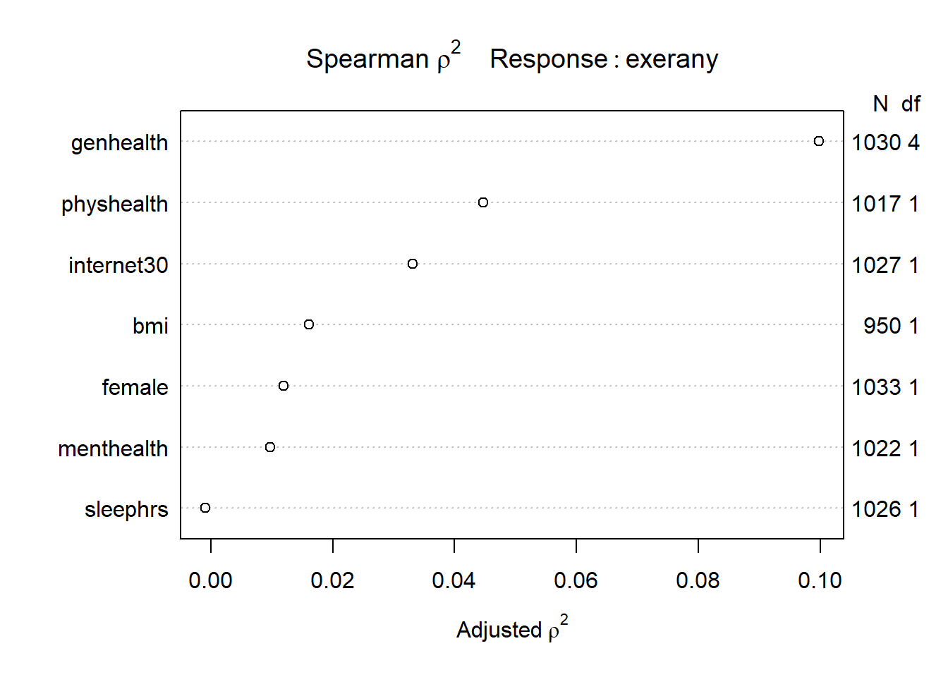
We see that the best candidate for a non-linear term is the genhealth variable, according to this plot, followed by the physhealth and internet30 predictors, then bmi. I will wind up fitting a model including the following non-linear terms…
- our pre-planned
femalexbmiandinternet30xgenhealthinteraction terms, - a new
genhealthxphyshealthinteraction term, - a restricted cubic spline with 5 knots for
physhealth - a restricted cubic spline with 4 knots for
bmi(so the interaction term withfemalewill need to account for this and restrict our interaction to the linear piece ofbmi)
14.5 A Second Model for exerany (Complete Cases)
Here’s the resulting model fit without worrying about imputation yet. This is just to make sure our code works. Note that I’m inserting the main effects of our interaction terms explicitly before including the interaction terms themselves, and that I need to use %ia% to include the interaction terms where one of the terms is included in the model with a spline. Again, I won’t draw any serious conclusions yet.
m2 <- lrm(exerany ~ rcs(bmi, 4) + rcs(physhealth, 5) +
              female + internet30 * genhealth +
              genhealth %ia% physhealth + female %ia% bmi +
              menthealth + sleephrs,
          data = smartcle1)
m2
Frequencies of Missing Values Due to Each Variable
exerany bmi physhealth female internet30 genhealth
3 84 17 0 6 3
menthealth sleephrs
11 8
Logistic Regression Model
lrm(formula = exerany ~ rcs(bmi, 4) + rcs(physhealth, 5) + female +
internet30 * genhealth + genhealth %ia% physhealth + female %ia%
bmi + menthealth + sleephrs, data = smartcle1)
Model Likelihood Discrimination Rank Discrim.
Ratio Test Indexes Indexes
Obs 924 LR chi2 142.51 R2 0.215 C 0.743
0 219 d.f. 22 g 1.053 Dxy 0.485
1 705 Pr(> chi2) <0.0001 gr 2.867 gamma 0.485
max |deriv| 6e-13 gp 0.178 tau-a 0.176
Brier 0.151
Coef S.E. Wald Z Pr(>|Z|)
Intercept 2.2998 1.9789 1.16 0.2452
bmi 0.0052 0.0801 0.06 0.9482
bmi' -0.2988 0.3555 -0.84 0.4006
bmi'' 0.8809 0.9615 0.92 0.3596
physhealth 0.0410 0.0868 0.47 0.6362
physhealth' -0.2944 0.3888 -0.76 0.4489
female -0.6307 0.8228 -0.77 0.4434
internet30 0.6722 0.7134 0.94 0.3460
genhealth=2_VeryGood -0.3092 0.7700 -0.40 0.6880
genhealth=3_Good -0.7559 0.7194 -1.05 0.2934
genhealth=4_Fair -1.1611 0.7646 -1.52 0.1289
genhealth=5_Poor -2.3680 1.2846 -1.84 0.0653
genhealth=2_VeryGood * physhealth 0.0099 0.0824 0.12 0.9043
genhealth=3_Good * physhealth -0.0406 0.0772 -0.53 0.5992
genhealth=4_Fair * physhealth -0.0407 0.0773 -0.53 0.5988
genhealth=5_Poor * physhealth 0.0534 0.0868 0.62 0.5382
female * bmi -0.0023 0.0275 -0.08 0.9324
menthealth -0.0143 0.0125 -1.15 0.2522
sleephrs -0.0457 0.0561 -0.81 0.4153
internet30 * genhealth=2_VeryGood 0.2174 0.8330 0.26 0.7941
internet30 * genhealth=3_Good 0.0375 0.7767 0.05 0.9615
internet30 * genhealth=4_Fair -0.3080 0.8371 -0.37 0.7129
internet30 * genhealth=5_Poor -1.9411 1.0150 -1.91 0.0558
plot(anova(m2))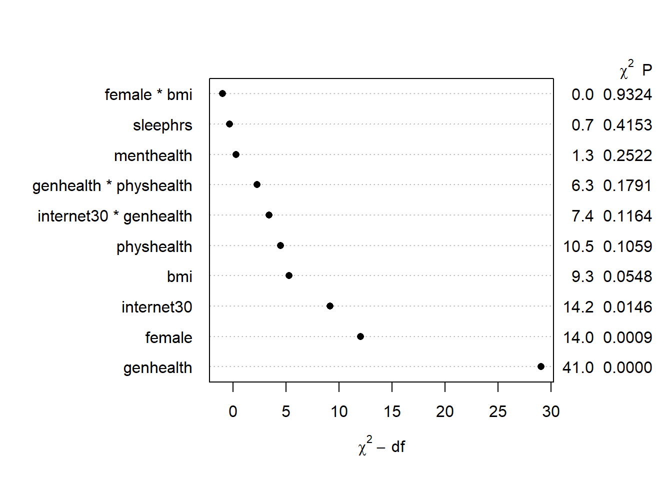
14.6 Dealing with Missing Data via Simple Imputation
One approach we might take in this problem is to use simple imputation to deal with our missing values. I will proceed as follows:
- Omit all cases where the outcome
exeranyis missing. - Determine (and plot) the remaining missingness.
- Use simple imputation for all predictors, and build a new data set with “complete” data.
- Re-fit the proposed models using this new data set.
14.6.1 Omit cases where the outcome is missing
We need to drop the cases where exerany is missing in smartcle1. We’ll begin creating an imputed data set, called smartcle_imp0, by filtering on complete data for exerany, as follows.
Hmisc::describe(smartcle1$exerany)smartcle1$exerany
n missing distinct Info Sum Mean Gmd
1033 3 2 0.546 786 0.7609 0.3642 smartcle_imp0 <- smartcle1 %>%
filter(complete.cases(exerany)) %>%
select(SEQNO, exerany, physhealth, menthealth,
genhealth, bmi, female, internet30, sleephrs)
Hmisc::describe(smartcle_imp0$exerany)smartcle_imp0$exerany
n missing distinct Info Sum Mean Gmd
1033 0 2 0.546 786 0.7609 0.3642 14.6.2 Plot the remaining missingness
We’ll look at the missing values (excluding the subject ID: SEQNO) in our new data set. Of course, we can get a count of missing values within each variable with skim or with:
colSums(is.na(smartcle_imp0)) SEQNO exerany physhealth menthealth genhealth bmi
0 0 16 11 3 83
female internet30 sleephrs
0 6 7 The Hmisc package has a plotting approach which can help identify missingness, too.
naplot(naclus(select(smartcle_imp0, -SEQNO)))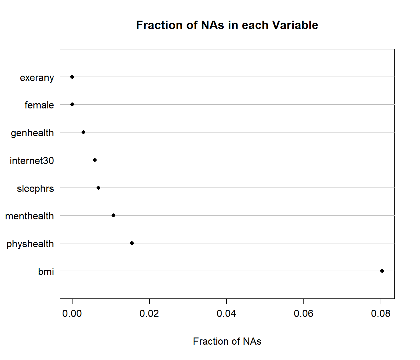
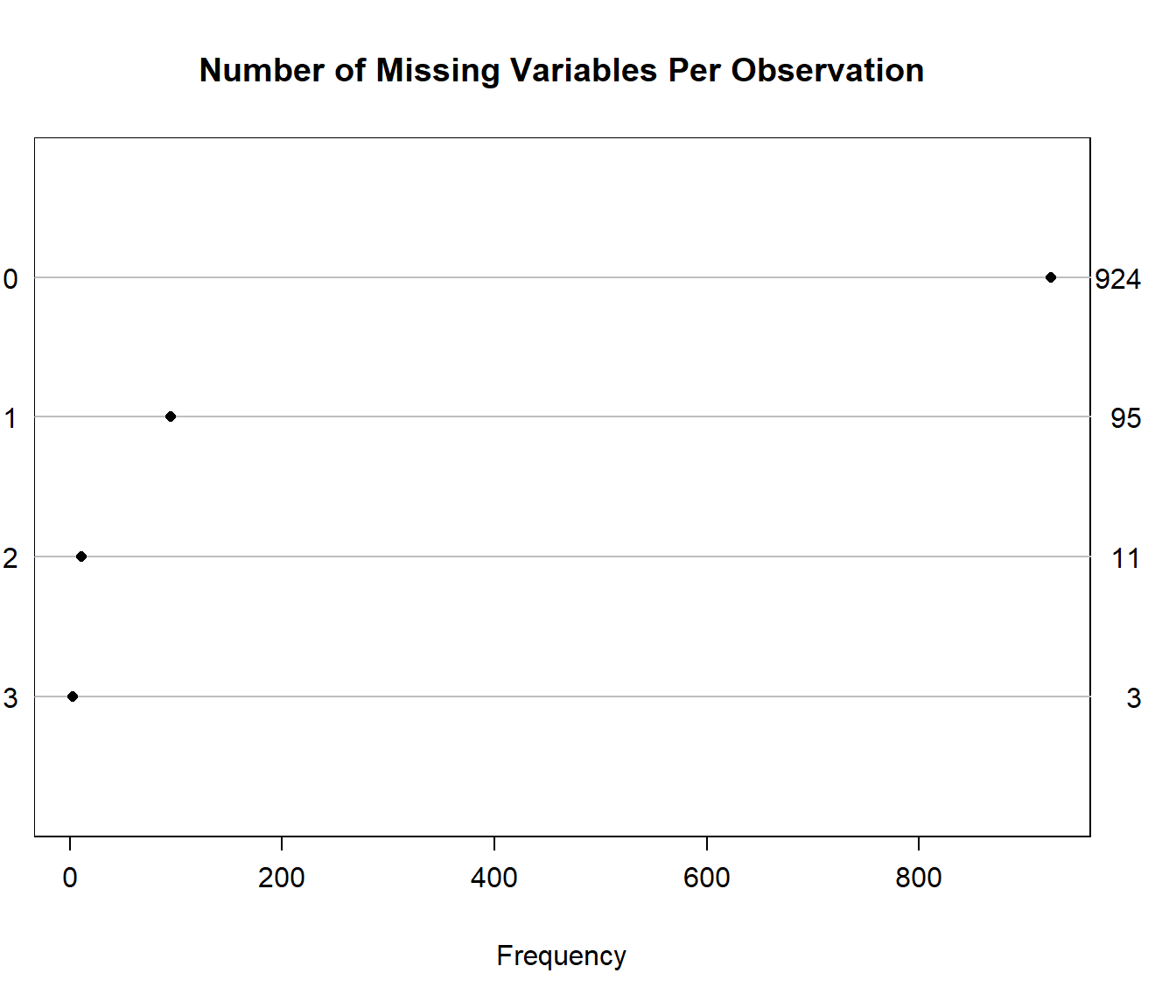
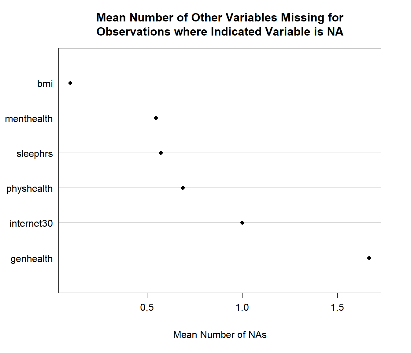
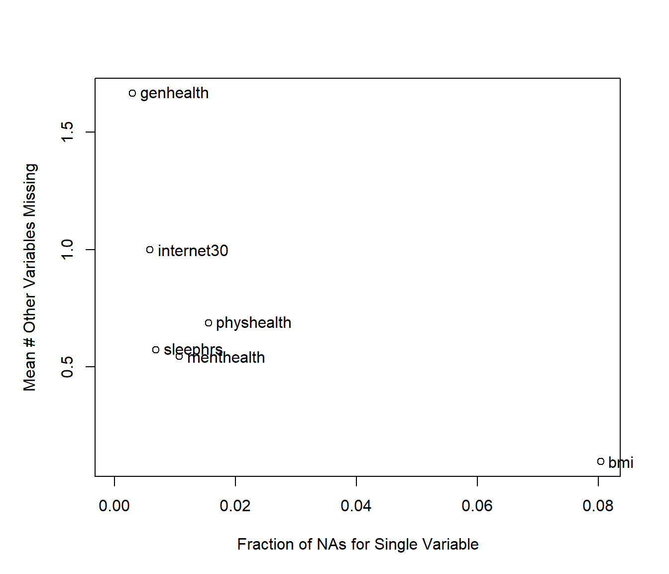
We can also get a useful accounting of missing data patterns, with the md.pattern function in the mice package.
mice::md.pattern(smartcle_imp0)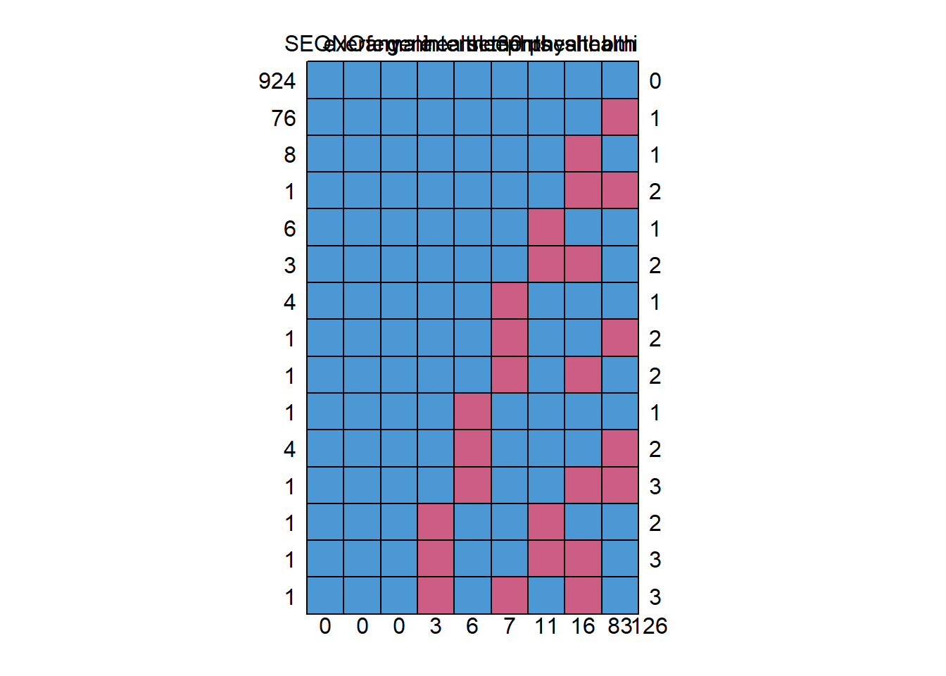
    SEQNO exerany female genhealth internet30 sleephrs menthealth
924     1       1      1         1          1        1          1
76      1       1      1         1          1        1          1
8       1       1      1         1          1        1          1
1       1       1      1         1          1        1          1
6       1       1      1         1          1        1          0
3       1       1      1         1          1        1          0
4       1       1      1         1          1        0          1
1       1       1      1         1          1        0          1
1       1       1      1         1          1        0          1
1       1       1      1         1          0        1          1
4       1       1      1         1          0        1          1
1       1       1      1         1          0        1          1
1       1       1      1         0          1        1          0
1       1       1      1         0          1        1          0
1       1       1      1         0          1        0          1
        0       0      0         3          6        7         11
    physhealth bmi
924          1   1   0
76           1   0   1
8            0   1   1
1            0   0   2
6            1   1   1
3            0   1   2
4            1   1   1
1            1   0   2
1            0   1   2
1            1   1   1
4            1   0   2
1            0   0   3
1            1   1   2
1            0   1   3
1            0   1   3
            16  83 126
We can also do this with na.pattern in the Hmisc package, but then we have to get the names of the columns, too, so that we can read off the values.
na.pattern(smartcle_imp0)pattern
000000000 000000001 000000010 000001000 000001001 000001010 000100000
924 4 1 76 1 4 6
000110000 001000000 001000001 001001000 001001010 001010001 001100000
1 8 1 1 1 1 3
001110000
1 names(smartcle_imp0)[1] "SEQNO" "exerany" "physhealth" "menthealth" "genhealth"
[6] "bmi" "female" "internet30" "sleephrs" 14.6.3 Use simple imputation, build a new data set
The only variables that require no imputation are exerany and female. In this case, we need to impute:
- 83
bmivalues (which are quantitative) - 16
physhealthvalues (quantitative, must fall between 0 and 30) - 11
menthealthvalues (quantitative, must fall between 0 and 30) - 7
sleephrsvalues (quantitative, must fall between 0 and 24) - 6
internet30values (which are 1/0) - and 3
genhealthvalues (which are multi-categorical, so we need to convert them to numbers in order to get the imputation process to work properly)
smartcle_imp0 <- smartcle_imp0 %>%
    mutate(genh_n = as.numeric(genhealth))

smartcle_imp0 %>% count(genhealth, genh_n)
Warning: Factor `genhealth` contains implicit NA, consider using
`forcats::fct_explicit_na`# A tibble: 6 x 3
genhealth genh_n n
<fct> <dbl> <int>
1 1_Excellent 1 172
2 2_VeryGood 2 350
3 3_Good 3 344
4 4_Fair 4 121
5 5_Poor 5 43
6 <NA> NA 3I’ll work from the bottom up, using various simputation functions to accomplish the imputations I want. In this case, I’ll use predictive mean matching for the categorical data, and linear models or elastic net approaches for the quantitative data. Be sure to set a seed beforehand so you can replicate your work.
set.seed(432234)

smartcle_imp1 <- smartcle_imp0 %>%
    impute_pmm(genh_n ~ female) %>%
    impute_pmm(internet30 ~ female + genh_n) %>%
    impute_lm(sleephrs ~ female + genh_n) %>%
    impute_lm(menthealth ~ female + sleephrs) %>%
    impute_en(physhealth ~ female + genh_n + sleephrs) %>%
    impute_en(bmi ~ physhealth + genh_n)
After the imputations are complete, I’ll back out of the numeric version of genhealth, called genh_n back to my original variable, then check to be sure I now have no missing values.
smartcle_imp1 <- smartcle_imp1 %>%
    mutate(genhealth = fct_recode(factor(genh_n),
                                  "1_Excellent" = "1",
                                  "2_VeryGood" = "2",
                                  "3_Good" = "3",
                                  "4_Fair" = "4",
                                  "5_Poor" = "5"))

smartcle_imp1 %>% count(genhealth, genh_n)
# A tibble: 5 x 3
genhealth genh_n n
<fct> <dbl> <int>
1 1_Excellent 1 172
2 2_VeryGood 2 351
3 3_Good 3 346
4 4_Fair 4 121
5 5_Poor 5 43colSums(is.na(smartcle_imp1)) SEQNO exerany physhealth menthealth genhealth bmi
0 0 0 0 0 0
female internet30 sleephrs genh_n
0 0 0 0 OK. Looks good. I now have a data frame called smartcle_imp1 with no missingness, which I can use to fit my logistic regression models. Let’s do that next, and then return to the problem of accounting for missingness through multiple imputation.
14.7 Refitting Model 1 with simply imputed data
Using the numeric version of the genhealth data, called genh_n, will ease the reviewing of later output, so we’ll do that here, making sure R knows that genh_n describes a categorical factor.
d <- datadist(smartcle_imp1)
options(datadist = "d")

m1_a <- lrm(exerany ~ internet30 * catg(genh_n) + bmi * female +
              physhealth + menthealth + sleephrs,
          data = smartcle_imp1, x = TRUE, y = TRUE)
m1_a
Logistic Regression Model
lrm(formula = exerany ~ internet30 * catg(genh_n) + bmi * female +
physhealth + menthealth + sleephrs, data = smartcle_imp1,
x = TRUE, y = TRUE)
Model Likelihood Discrimination Rank Discrim.
Ratio Test Indexes Indexes
Obs 1033 LR chi2 151.09 R2 0.204 C 0.741
0 247 d.f. 15 g 1.023 Dxy 0.482
1 786 Pr(> chi2) <0.0001 gr 2.780 gamma 0.483
max |deriv| 1e-12 gp 0.175 tau-a 0.176
Brier 0.154
Coef S.E. Wald Z Pr(>|Z|)
Intercept 3.3390 0.9731 3.43 0.0006
internet30 0.6487 0.7010 0.93 0.3548
genh_n=2 -0.4938 0.7459 -0.66 0.5080
genh_n=3 -0.9270 0.6972 -1.33 0.1836
genh_n=4 -1.3060 0.7378 -1.77 0.0767
genh_n=5 -0.8093 0.8329 -0.97 0.3312
bmi -0.0412 0.0217 -1.90 0.0570
female -0.9473 0.7722 -1.23 0.2199
physhealth -0.0229 0.0102 -2.25 0.0246
menthealth -0.0200 0.0114 -1.76 0.0784
sleephrs -0.0415 0.0492 -0.84 0.3994
internet30 * genh_n=2 0.3701 0.8065 0.46 0.6463
internet30 * genh_n=3 0.1295 0.7543 0.17 0.8637
internet30 * genh_n=4 -0.2194 0.8108 -0.27 0.7867
internet30 * genh_n=5 -1.4080 0.9636 -1.46 0.1440
bmi * female 0.0118 0.0261 0.45 0.6497
All right. We’ve used 1033 observations, which is correct (after deleting the three with missing exerany.) The model shows a Nagelkerke R2 value of 0.204, and a C statistic of 0.741 after imputation. The likelihood ratio (drop in deviance) test is highly significant.
14.7.1 Validating Summary Statistics
set.seed(432099)
validate(m1_a)
index.orig training test optimism index.corrected n
Dxy 0.4823 0.5012 0.4632 0.0380 0.4444 40
R2 0.2039 0.2218 0.1878 0.0340 0.1699 40
Intercept 0.0000 0.0000 0.0936 -0.0936 0.0936 40
Slope 1.0000 1.0000 0.9001 0.0999 0.9001 40
Emax 0.0000 0.0000 0.0401 0.0401 0.0401 40
D 0.1453 0.1592 0.1329 0.0264 0.1189 40
U -0.0019 -0.0019 0.0013 -0.0032 0.0013 40
Q 0.1472 0.1612 0.1316 0.0295 0.1177 40
B 0.1539 0.1507 0.1566 -0.0058 0.1597 40
g 1.0226 1.0868 0.9722 0.1146 0.9080 40
gp 0.1751 0.1818 0.1673 0.0145 0.1606 40It appears that the model’s description of summary statistics is a little optimistic for both the C statistic (remember that C = 0.5 + Dxy/2) and the Nagelkerke R2. This output suggests that in a new sample of data, our model might be better expected to show a C statistic near …
\[ C = 0.5 + \frac{Dxy}{2} = 0.5 + \frac{0.4444}{2} = 0.7222 \]
rather than the 0.741 we saw initially, and that the Nagelkerke R2 in new data will be closer to 0.17, than to the nominal 0.204 we saw above. So, as we walk through some other output for this model, remember that the C statistic wasn’t great here (0.72 after validation), so our ability to discriminate exercisers from non-exercisers is still a problem.
14.7.2 ANOVA for the model
Next, let’s look at the ANOVA comparisons for this model.
anova(m1_a) Wald Statistics Response: exerany
Factor Chi-Square d.f. P
internet30 (Factor+Higher Order Factors) 17.28 5 0.0040
All Interactions 5.84 4 0.2116
genh_n (Factor+Higher Order Factors) 35.81 8 <.0001
All Interactions 5.84 4 0.2116
bmi (Factor+Higher Order Factors) 7.36 2 0.0252
All Interactions 0.21 1 0.6497
female (Factor+Higher Order Factors) 12.72 2 0.0017
All Interactions 0.21 1 0.6497
physhealth 5.05 1 0.0246
menthealth 3.10 1 0.0784
sleephrs 0.71 1 0.3994
internet30 * genh_n (Factor+Higher Order Factors) 5.84 4 0.2116
bmi * female (Factor+Higher Order Factors) 0.21 1 0.6497
TOTAL INTERACTION 6.15 5 0.2917
TOTAL 126.95 15 <.0001plot(anova(m1_a))
It looks like several of the variables (genhealth, internet30, female, bmi and physhealth) are carrying statistically significant predictive value here.
We can also build a plot of the AIC values attributable to each piece of the model.
plot(anova(m1_a), what="aic")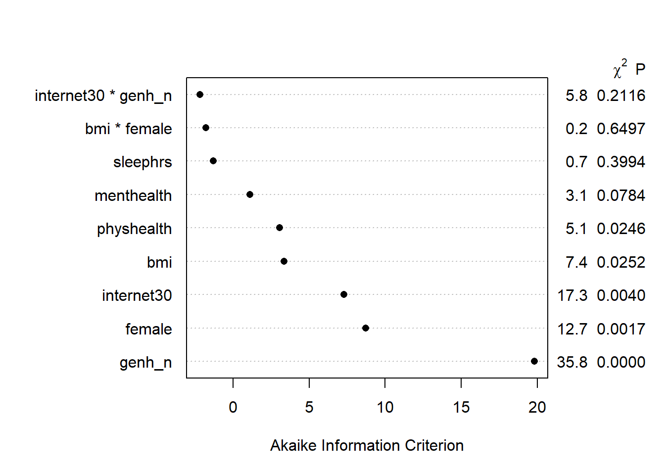
14.7.3 Summarizing Effect Size
How big are the effects we see?
plot(summary(m1_a))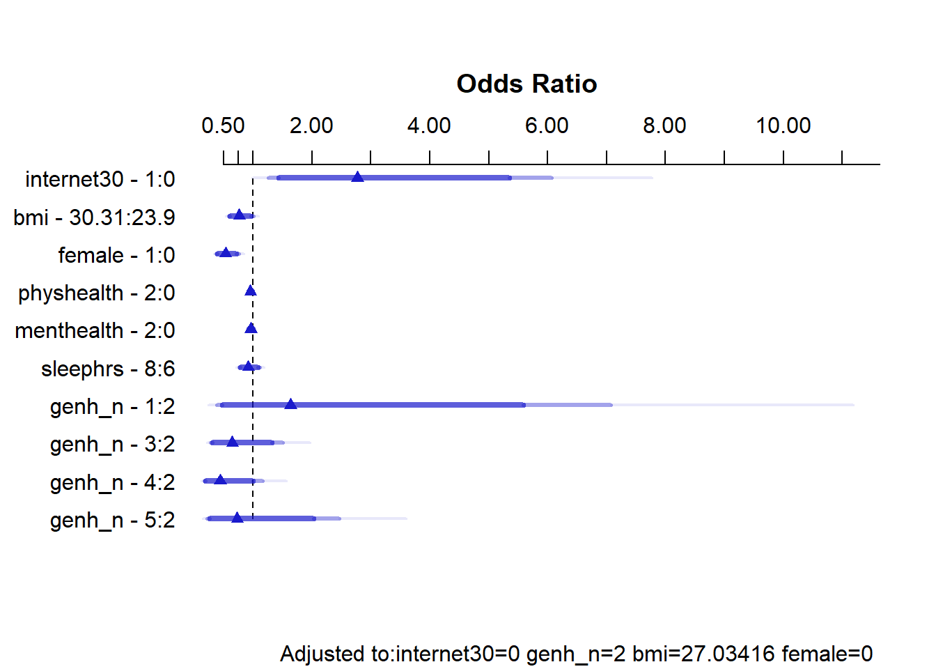
summary(m1_a) Effects Response : exerany
Factor Low High Diff. Effect S.E. Lower 0.95 Upper 0.95
internet30 0.0 1.00 1.00 1.018800 0.400350 0.234160 1.8035000
Odds Ratio 0.0 1.00 1.00 2.770000 NA 1.263800 6.0710000
bmi 23.9 30.31 6.41 -0.264180 0.138810 -0.536240 0.0078783
Odds Ratio 23.9 30.31 6.41 0.767840 NA 0.584950 1.0079000
female 0.0 1.00 1.00 -0.627270 0.177840 -0.975830 -0.2787200
Odds Ratio 0.0 1.00 1.00 0.534050 NA 0.376880 0.7567500
physhealth 0.0 2.00 2.00 -0.045843 0.020393 -0.085813 -0.0058727
Odds Ratio 0.0 2.00 2.00 0.955190 NA 0.917770 0.9941400
menthealth 0.0 2.00 2.00 -0.040089 0.022778 -0.084733 0.0045549
Odds Ratio 0.0 2.00 2.00 0.960700 NA 0.918760 1.0046000
sleephrs 6.0 8.00 2.00 -0.082947 0.098439 -0.275880 0.1099900
Odds Ratio 6.0 8.00 2.00 0.920400 NA 0.758900 1.1163000
genh_n - 1:2 2.0 1.00 NA 0.493760 0.745930 -0.968240 1.9558000
Odds Ratio 2.0 1.00 NA 1.638500 NA 0.379750 7.0693000
genh_n - 3:2 2.0 3.00 NA -0.433290 0.431840 -1.279700 0.4131100
Odds Ratio 2.0 3.00 NA 0.648370 NA 0.278120 1.5115000
genh_n - 4:2 2.0 4.00 NA -0.812200 0.490270 -1.773100 0.1487200
Odds Ratio 2.0 4.00 NA 0.443880 NA 0.169800 1.1603000
genh_n - 5:2 2.0 5.00 NA -0.315510 0.620110 -1.530900 0.8998700
Odds Ratio 2.0 5.00 NA 0.729420 NA 0.216340 2.4593000
Adjusted to: internet30=0 genh_n=2 bmi=27.03416 female=0 This output is easier to read as a result of using small numeric labels in genh_n, rather than the lengthy labels in genhealth. The sensible things to interpret are the odds ratios.
- holding all other predictors constant, the effect of moving from
internet30= 0 tointernet30= 1 is that the odds ofexeranyincrease by a factor of 2.77.- Suppose Harry and Steve have the same values of all predictors in this model except that Harry used the internet and Steve did not.
- So the odds of exercising for Harry (who used the internet) are 2.77 times higher than the odds of exercising for Steve (who didn’t use the internet), assuming that all other predictors are the same.
- We also have a 95% confidence interval for this odds ratio, which is (1.26, 6.07). Since 1 is not in that interval, the data don’t seem to be consistent with
internet30having no effect onexerany.
- the odds ratio comparing two subjects with the same predictors except that Harry has a BMI of 30.31 (the 75th percentile of observed BMIs in our sample) and Marty has a BMI of 23.9 (the 25th percentile) is that Harry has 0.767 times the odds of exercising that Marty does. So Harry’s probability of exercise will also be lower than Marty’s.
- The 95% confidence interval in this case is (0.58, 1.01), and because 1 is in that interval, we cannot conclude that the effect of
bmimeets the standard for statistical significance at the 5% level.
- The 95% confidence interval in this case is (0.58, 1.01), and because 1 is in that interval, we cannot conclude that the effect of
- A similar approach can be used to describe the odds ratios associated with each predictor.
- Note that each of the categories in
genh_nis compared to a single baseline category. Here, that’s category 2. R will pick the modal category: the one that appears most often in the data. The comparisons of each category against category 2 are not significant in each case, at the 5% level.
14.7.4 Plotting the Model with ggplot and Predict
Let’s look at a series of plots describing the model on the probability scale.
ggplot(Predict(m1_a, fun = plogis))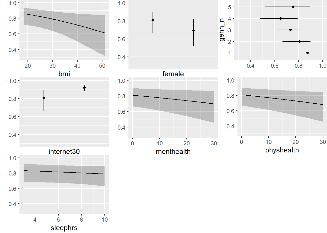
This helps us describe what is happening in terms of direction at least. For example,
- As
bmiincreases, predicted Pr(exerany) decreases. - People who accessed the internet in the past 30 days have higher model probabilities of exercising.
Do any of these plots fail to make sense to you? Is anything moving in a surprising direction?
14.7.5 Plotting the model with a nomogram
plot(nomogram(m1_a, fun = plogis))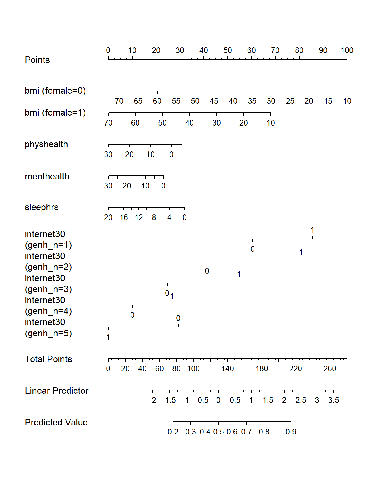
Note the impact of our interaction terms, and how we have two lines for bmi and five lines for internet30 that come out of our product terms. As with any nomogram, to make a prediction we:
- find the values of each of our predictors in the scales, and travel vertically up to the Points line to read off the Points for that predictor.
- sum up the Points across all predictors, and find that location in the Total Points line.
- move vertically down from the total points line to find the estimated “linear predictor” (log odds ratio) and finally the “predicted value” (probability of our outcome
exerany= 1.)
14.7.6 Checking the Goodness of Fit of our model
To test the goodness of fit, we can use the following omnibus test:
round(residuals(m1_a, type = "gof"),3)Sum of squared errors Expected value|H0 SD
158.955 158.740 0.525
Z P
0.408 0.683 Our non-significant p value suggests that we cannot detect anything that’s obviously wrong in the model in terms of goodness of fit. That’s comforting.
14.8 Refitting Model 2 with simply imputed data
I’ll walk through the same tasks for Model m2 that I did above for Model m1. Again, we’re running this model after simple imputation of missing values.
Using the numeric version of the genhealth data, called genh_n, will ease the reviewing of later output, so we’ll do that here, making sure R knows that genh_n describes a categorical factor.
d <- datadist(smartcle_imp1)
options(datadist = "d")

m2_a <- lrm(exerany ~ rcs(bmi, 4) + rcs(physhealth, 5) +
              female + internet30 * catg(genh_n) +
              catg(genh_n) %ia% physhealth + female %ia% bmi +
              menthealth + sleephrs,
          data = smartcle_imp1, x = TRUE, y = TRUE)
m2_a
Logistic Regression Model
lrm(formula = exerany ~ rcs(bmi, 4) + rcs(physhealth, 5) + female +
internet30 * catg(genh_n) + catg(genh_n) %ia% physhealth +
female %ia% bmi + menthealth + sleephrs, data = smartcle_imp1,
x = TRUE, y = TRUE)
Model Likelihood Discrimination Rank Discrim.
Ratio Test Indexes Indexes
Obs 1033 LR chi2 159.51 R2 0.214 C 0.744
0 247 d.f. 22 g 1.051 Dxy 0.487
1 786 Pr(> chi2) <0.0001 gr 2.860 gamma 0.487
max |deriv| 4e-12 gp 0.179 tau-a 0.177
Brier 0.152
Coef S.E. Wald Z Pr(>|Z|)
Intercept 2.7525 1.9074 1.44 0.1490
bmi -0.0072 0.0763 -0.09 0.9250
bmi' -0.2772 0.3288 -0.84 0.3992
bmi'' 0.9199 0.9873 0.93 0.3515
physhealth 0.0287 0.0905 0.32 0.7514
physhealth' -0.1396 0.3555 -0.39 0.6946
female -0.9550 0.8017 -1.19 0.2336
internet30 0.6099 0.7040 0.87 0.3863
genh_n=2 -0.5059 0.7507 -0.67 0.5004
genh_n=3 -0.8611 0.7053 -1.22 0.2221
genh_n=4 -1.1827 0.7535 -1.57 0.1165
genh_n=5 -2.6842 1.1987 -2.24 0.0251
genh_n=2 * physhealth -0.0253 0.0864 -0.29 0.7698
genh_n=3 * physhealth -0.0475 0.0842 -0.56 0.5723
genh_n=4 * physhealth -0.0471 0.0842 -0.56 0.5758
genh_n=5 * physhealth 0.0497 0.0917 0.54 0.5879
female * bmi 0.0111 0.0268 0.41 0.6803
menthealth -0.0200 0.0116 -1.72 0.0859
sleephrs -0.0536 0.0503 -1.07 0.2868
internet30 * genh_n=2 0.4193 0.8091 0.52 0.6043
internet30 * genh_n=3 0.1624 0.7592 0.21 0.8306
internet30 * genh_n=4 -0.1802 0.8176 -0.22 0.8255
internet30 * genh_n=5 -1.6615 0.9820 -1.69 0.0907
All right. We’ve again used 1033 observations, which is correct (after deleting the three with missing exerany. The model shows a Nagelkerke R2 value of 0.214, and a C statistic of 0.744 after imputation. Each of these results are a little better than what we saw with m1_a but only a little. The likelihood ratio (drop in deviance) test is still highly significant.
14.8.1 Validating Summary Statistics
set.seed(432009)
validate(m2_a)
index.orig training test optimism index.corrected n
Dxy 0.4870 0.5058 0.4590 0.0468 0.4402 40
R2 0.2145 0.2340 0.1849 0.0491 0.1654 40
Intercept 0.0000 0.0000 0.1729 -0.1729 0.1729 40
Slope 1.0000 1.0000 0.8473 0.1527 0.8473 40
Emax 0.0000 0.0000 0.0692 0.0692 0.0692 40
D 0.1534 0.1695 0.1307 0.0387 0.1147 40
U -0.0019 -0.0019 0.0041 -0.0060 0.0041 40
Q 0.1554 0.1714 0.1266 0.0448 0.1106 40
B 0.1521 0.1502 0.1567 -0.0065 0.1585 40
g 1.0507 1.1335 0.9626 0.1708 0.8799 40
gp 0.1786 0.1866 0.1642 0.0224 0.1562 40Again, the model’s description of summary statistics is a little optimistic for both the C statistic and the Nagelkerke R2. In a new sample of data, model m2_a might be better expected to show a C statistic near …
\[ C = 0.5 + \frac{Dxy}{2} = 0.5 + \frac{0.4402}{2} = 0.7201 \]
rather than the 0.744 we saw initially, and that the Nagelkerke R2 in new data will be closer to 0.165, than to the nominal 0.215 we saw above. So, after validation, this model actually looks worse than model m1_a.
| Model | nominal C | nominal R2 | validated C | validated R2 |
|---|---|---|---|---|
m1_a |
0.741 | 0.204 | 0.722 | 0.170 |
m2_a |
0.744 | 0.214 | 0.720 | 0.165 |
Again, as we walk through other output for model m2_a, remember that the our ability to discriminate exercisers from non-exercisers is still very much in question using either model.
14.8.2 ANOVA for the model
Next, let’s look at the ANOVA comparisons for this model.
anova(m2_a) Wald Statistics Response: exerany
Factor Chi-Square d.f. P
bmi (Factor+Higher Order Factors) 9.39 4 0.0521
All Interactions 0.17 1 0.6803
Nonlinear 1.46 2 0.4831
physhealth (Factor+Higher Order Factors) 11.74 6 0.0680
All Interactions 6.33 4 0.1760
Nonlinear 0.15 1 0.6946
female (Factor+Higher Order Factors) 13.25 2 0.0013
All Interactions 0.17 1 0.6803
internet30 (Factor+Higher Order Factors) 18.03 5 0.0029
All Interactions 7.49 4 0.1121
genh_n (Factor+Higher Order Factors) 39.00 12 0.0001
All Interactions 11.80 8 0.1604
genh_n * physhealth (Factor+Higher Order Factors) 6.33 4 0.1760
female * bmi (Factor+Higher Order Factors) 0.17 1 0.6803
menthealth 2.95 1 0.0859
sleephrs 1.13 1 0.2868
internet30 * genh_n (Factor+Higher Order Factors) 7.49 4 0.1121
TOTAL NONLINEAR 1.65 3 0.6474
TOTAL INTERACTION 12.10 9 0.2075
TOTAL NONLINEAR + INTERACTION 13.40 12 0.3409
TOTAL 131.03 22 <.0001plot(anova(m2_a))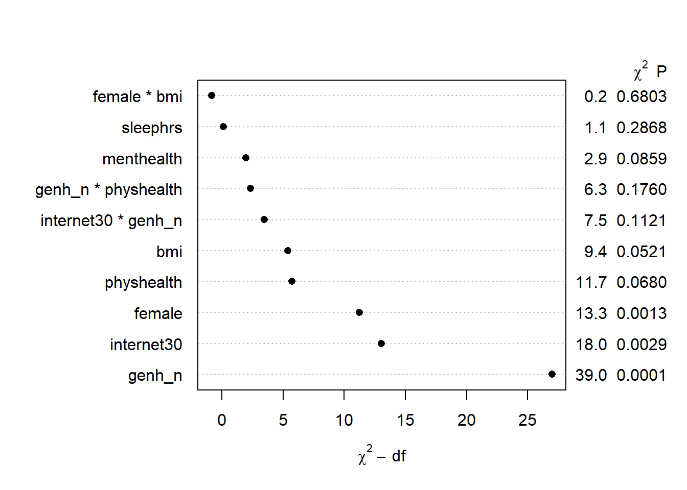
Here, it looks like just three of the variables (genhealth, internet30, and female) are carrying statistically significant predictive value.
Here is the AIC plot.
plot(anova(m2_a), what="aic")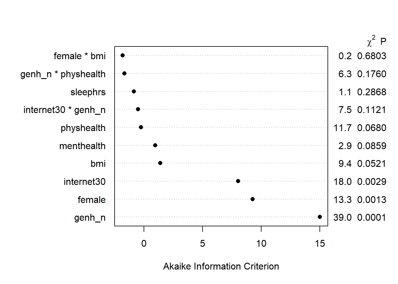
14.8.3 Summarizing Effect Size
How big are the effects we see?
plot(summary(m2_a))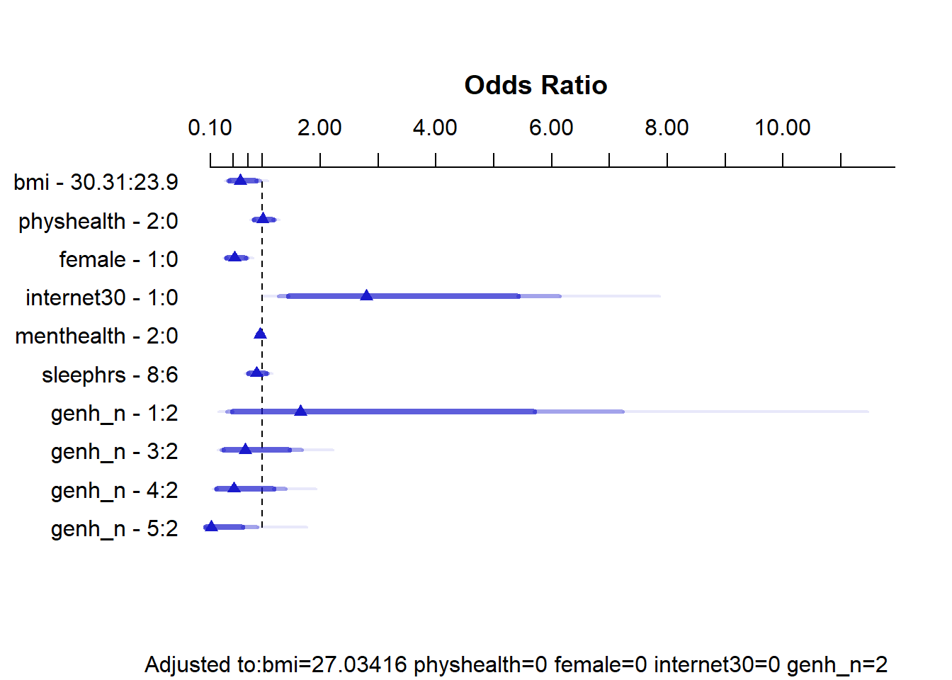
summary(m2_a) Effects Response : exerany
Factor Low High Diff. Effect S.E. Lower 0.95 Upper 0.95
bmi 23.9 30.31 6.41 -0.4797500 0.221460 -0.913810 -0.045691
Odds Ratio 23.9 30.31 6.41 0.6189400 NA 0.400990 0.955340
physhealth 0.0 2.00 2.00 0.0055399 0.095955 -0.182530 0.193610
Odds Ratio 0.0 2.00 2.00 1.0056000 NA 0.833160 1.213600
female 0.0 1.00 1.00 -0.6558700 0.183810 -1.016100 -0.295600
Odds Ratio 0.0 1.00 1.00 0.5189900 NA 0.361990 0.744080
internet30 0.0 1.00 1.00 1.0291000 0.401140 0.242910 1.815300
Odds Ratio 0.0 1.00 1.00 2.7986000 NA 1.275000 6.143200
menthealth 0.0 2.00 2.00 -0.0399460 0.023258 -0.085530 0.005638
Odds Ratio 0.0 2.00 2.00 0.9608400 NA 0.918030 1.005700
sleephrs 6.0 8.00 2.00 -0.1072500 0.100690 -0.304600 0.090096
Odds Ratio 6.0 8.00 2.00 0.8983000 NA 0.737420 1.094300
genh_n - 1:2 2.0 1.00 NA 0.5059000 0.750690 -0.965430 1.977200
Odds Ratio 2.0 1.00 NA 1.6585000 NA 0.380820 7.222700
genh_n - 3:2 2.0 3.00 NA -0.3552100 0.447130 -1.231600 0.521140
Odds Ratio 2.0 3.00 NA 0.7010200 NA 0.291830 1.684000
genh_n - 4:2 2.0 4.00 NA -0.6768400 0.517450 -1.691000 0.337350
Odds Ratio 2.0 4.00 NA 0.5082200 NA 0.184330 1.401200
genh_n - 5:2 2.0 5.00 NA -2.1783000 1.066000 -4.267700 -0.089045
Odds Ratio 2.0 5.00 NA 0.1132300 NA 0.014015 0.914800
Adjusted to: bmi=27.03416 physhealth=0 female=0 internet30=0 genh_n=2 This output is easier to read as a result of using small numeric labels in genh_n, rather than the lengthy labels in genhealth. The sensible things to interpret are the odds ratios. For example,
- holding all other predictors constant, the effect of moving from
internet30= 0 tointernet30= 1 is that the odds ofexeranyincrease by a factor of 2.80. - the odds ratio comparing two subjects with the same predictors except that Harry has a BMI of 30.31 (the 75th percentile of observed BMIs in our sample) and Marty has a BMI of 23.9 (the 25th percentile) is that Harry has 0.619 times the odds of exercising that Marty does. So Harry’s probability of exercise will also be lower.
By sex, which group has a larger probability of exerany, holding all other predictors constant, by this model? Females or Males?
14.8.4 Plotting the Model with ggplot and Predict
Again, consider a series of plots describing the model m2_a on the probability scale.
ggplot(Predict(m2_a, fun = plogis))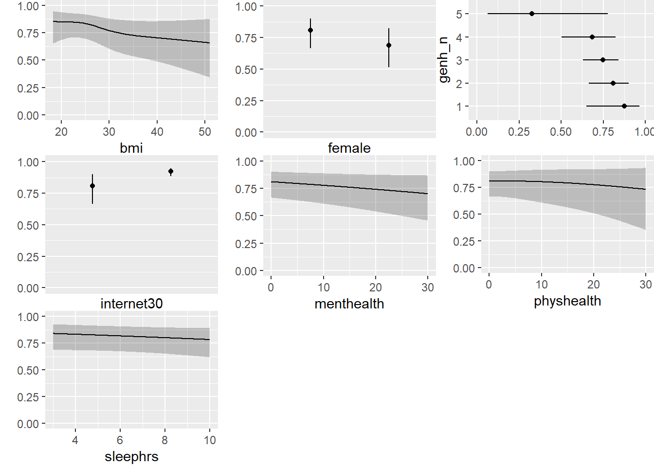
Note the small kink in the bmi plot. To what do you attribute this?
14.8.5 Plotting the model with a nomogram
plot(nomogram(m2_a, fun = plogis))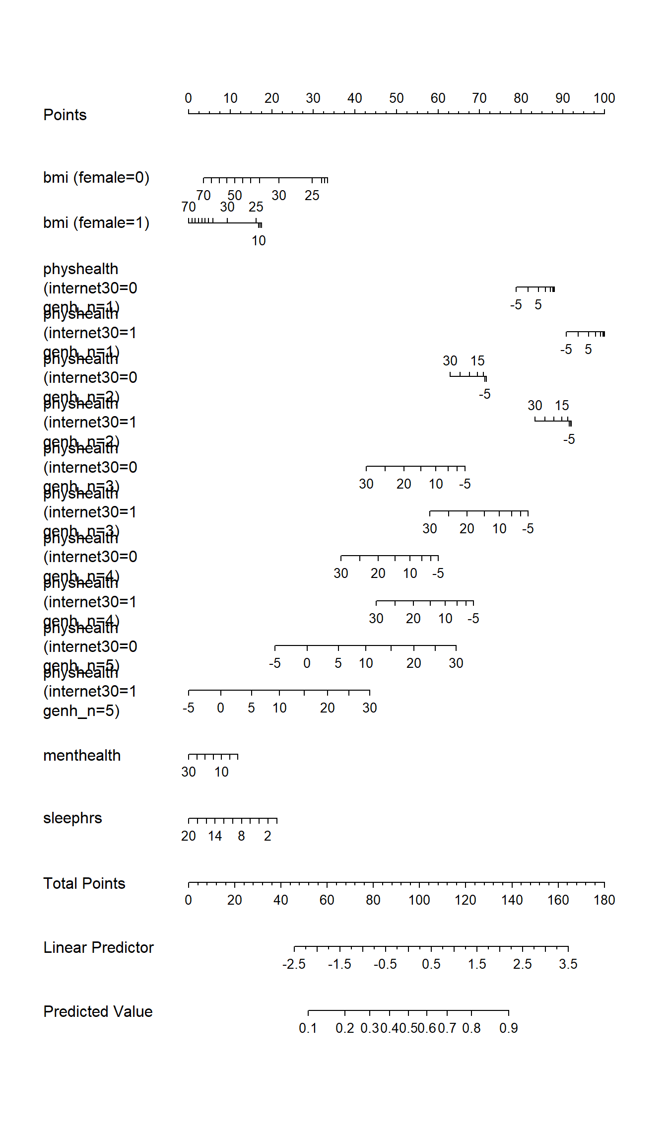
Note the impact of our interaction terms, and the cubic splines in bmi and physhealth. As with any nomogram, to make a prediction we:
- find the values of each of our predictors in the scales, and travel vertically up to the Points line to read off the Points for that predictor.
- sum up the Points across all predictors, and find that location in the Total Points line.
- move vertically down from the total points line to find the estimated “linear predictor” (log odds ratio) and finally the “predicted value” (probability of our outcome
exerany= 1.)
14.8.6 Checking the Goodness of Fit of our model
To test the goodness of fit, we can use the following omnibus test:
round(residuals(m2_a, type = "gof"),3)Sum of squared errors Expected value|H0 SD
157.102 157.011 0.522
Z P
0.174 0.862 Our non-significant p value suggests that we cannot detect anything that’s obviously wrong in the model in terms of goodness of fit.
14.9 Comparing Model 2 to Model 1 after simple imputation
We can refit the models with glm and then compare them with anova, aic and bic approaches, if we like.
m1_a_glm <- glm(exerany ~ internet30 * factor(genh_n) +
                    bmi * female + physhealth + menthealth +
                    sleephrs,
                data = smartcle_imp1,
                family = binomial)

m2_a_glm <- glm(exerany ~ rcs(bmi, 4) + rcs(physhealth, 5) +
              female + internet30 * factor(genh_n) +
              factor(genh_n) %ia% physhealth + female %ia% bmi +
              menthealth + sleephrs,
          data = smartcle_imp1,
          family = binomial)
14.9.1 Comparison by Analysis of Deviance
anova(m1_a_glm, m2_a_glm)Analysis of Deviance Table
Model 1: exerany ~ internet30 * factor(genh_n) + bmi * female + physhealth +
menthealth + sleephrs
Model 2: exerany ~ rcs(bmi, 4) + rcs(physhealth, 5) + female + internet30 *
factor(genh_n) + factor(genh_n) %ia% physhealth + female %ia%
bmi + menthealth + sleephrs
Resid. Df Resid. Dev Df Deviance
1 1017 985.32
2 1010 976.89 7 8.4245To obtain a p value, we can compare this drop in deviance to a \(\chi^2\) distribution with 7 df, as follows:
pchisq(8.4245, 7, lower.tail = FALSE)[1] 0.2966531So there’s no statistically significant advantage apparent from fitting the larger m2_a model.
14.9.2 Comparing AIC and BIC
glance(m1_a_glm)# A tibble: 1 x 7
null.deviance df.null logLik AIC BIC deviance df.residual
<dbl> <int> <dbl> <dbl> <dbl> <dbl> <int>
1 1136. 1032 -493. 1017. 1096. 985. 1017glance(m2_a_glm)# A tibble: 1 x 7
null.deviance df.null logLik AIC BIC deviance df.residual
<dbl> <int> <dbl> <dbl> <dbl> <dbl> <int>
1 1136. 1032 -488. 1023. 1137. 977. 1010Model m1_a_glm shows lower AIC and BIC than does m2_a_glm, again suggesting no meaningful advantage for the larger model.
14.10 Dealing with Missing Data via Multiple Imputation
Next, we’ll use the aregImpute function within the Hmisc package to predict all missing values for all of our variables, using additive regression bootstrapping and predictive mean matching. The steps for this work are as follows:
aregImputedraws a sample with replacement from the observations where the target variable is observed, not missing.aregImputethen fits a flexible additive model to predict this target variable while finding the optimum transformation of it.aregImputethen uses this fitted flexible model to predict the target variable in all of the original observations.- Finally,
aregImputeimputes each missing value of the target variable with the observed value whose predicted transformed value is closest to the predicted transformed value of the missing value.
We’ll start with the smartcle_imp0 data set, which contains only the subjects in the original smartcle1 data where exerany is available, and which includes only the variables of interest to us, including both the factor (genhealth) and numeric (genh_n) versions of the genhealth data.
summary(smartcle_imp0) SEQNO exerany physhealth menthealth
Min. :2.016e+09 Min. :0.0000 Min. : 0.000 Min. : 0.000
1st Qu.:2.016e+09 1st Qu.:1.0000 1st Qu.: 0.000 1st Qu.: 0.000
Median :2.016e+09 Median :1.0000 Median : 0.000 Median : 0.000
Mean :2.016e+09 Mean :0.7609 Mean : 3.949 Mean : 2.701
3rd Qu.:2.016e+09 3rd Qu.:1.0000 3rd Qu.: 2.000 3rd Qu.: 2.000
Max. :2.016e+09 Max. :1.0000 Max. :30.000 Max. :30.000
NA's :16 NA's :11
genhealth bmi female internet30
1_Excellent:172 Min. :12.71 Min. :0.0000 Min. :0.0000
2_VeryGood :350 1st Qu.:23.70 1st Qu.:0.0000 1st Qu.:1.0000
3_Good :344 Median :26.68 Median :1.0000 Median :1.0000
4_Fair :121 Mean :27.85 Mean :0.6012 Mean :0.8101
5_Poor : 43 3rd Qu.:30.53 3rd Qu.:1.0000 3rd Qu.:1.0000
NA's : 3 Max. :66.06 Max. :1.0000 Max. :1.0000
NA's :83 NA's :6
sleephrs genh_n
Min. : 1.000 Min. :1.000
1st Qu.: 6.000 1st Qu.:2.000
Median : 7.000 Median :2.000
Mean : 7.022 Mean :2.527
3rd Qu.: 8.000 3rd Qu.:3.000
Max. :20.000 Max. :5.000
NA's :7 NA's :3 The smartcle_imp0 data set contains 1033 rows (subjects) and 10 columns (variables.)
14.10.1 Using aregImpute to fit a multiple imputation model
To set up aregImpute here, we’ll need to specify:
- a suitable random seed with
set.seedso we can replicate our work later - a data set via the
datadiststuff shown below - the variables we want to include in the imputation process, which should include, at a minimum, any variables with missing values, and any variables we want to include in our outcome models
n.impute= number of imputations, we’ll run 20 here10nk= number of knots to describe level of complexity, with our choicenk = c(0, 3)we’ll fit both linear models and models with restricted cubic splines with 3 knots (this approach will wind up throwing some warnings here because some of our variables with missing values have only a few options so fitting splines is tough.)tlinear = FALSEallows the target variable for imputation to have a non-linear transformation whennkis 3 or more. Here, I’ll usetlinear = TRUE, the default.B = 10specifies 10 bootstrap samples will be usedpr = FALSEtells the machine not to print out which iteration is running as it goes.dataspecifies the source of the variables
set.seed(432074)
dd <- datadist(smartcle_imp0)
options(datadist = "dd")

imp_fit <- aregImpute(~ exerany + physhealth + menthealth +
                          genh_n + bmi + female +
                          internet30 + sleephrs,
                   nk = c(0, 3), tlinear = TRUE,
                   data = smartcle_imp0, B = 10,
                   n.impute = 20, pr = FALSE)
OK. Here is the imputation model. The summary here isn’t especially critical. We want to see what was run, but to see what the results look like, we’ll need a plot, to come.
imp_fit
Multiple Imputation using Bootstrap and PMM

aregImpute(formula = ~exerany + physhealth + menthealth + genh_n +
    bmi + female + internet30 + sleephrs, data = smartcle_imp0,
    n.impute = 20, nk = c(0, 3), tlinear = TRUE, pr = FALSE,
    B = 10)

n: 1033     p: 8    Imputations: 20     nk: 0

Number of NAs:
   exerany physhealth menthealth     genh_n        bmi     female
         0         16         11          3         83          0
internet30   sleephrs
         6          7

           type d.f.
exerany       l    1
physhealth    s    1
menthealth    s    1
genh_n        s    1
bmi           s    1
female        l    1
internet30    l    1
sleephrs      s    1

Transformation of Target Variables Forced to be Linear

R-squares for Predicting Non-Missing Values for Each Variable
Using Last Imputations of Predictors
physhealth menthealth     genh_n        bmi internet30   sleephrs
     0.336      0.107      0.304      0.127      0.111      0.056

Resampling results for determining the complexity of imputation models

Variable being imputed: physhealth
                                         nk=0  nk=3
Bootstrap bias-corrected R^2            0.289 0.399
10-fold cross-validated  R^2            0.288 0.381
Bootstrap bias-corrected mean   |error| 4.911 4.014
10-fold cross-validated  mean   |error| 4.253 4.091
Bootstrap bias-corrected median |error| 3.261 1.784
10-fold cross-validated  median |error| 0.896 0.666

Variable being imputed: menthealth
                                         nk=0  nk=3
Bootstrap bias-corrected R^2            0.103 0.116
10-fold cross-validated  R^2            0.110 0.128
Bootstrap bias-corrected mean   |error| 3.660 3.651
10-fold cross-validated  mean   |error| 3.018 3.075
Bootstrap bias-corrected median |error| 1.957 1.780
10-fold cross-validated  median |error| 0.715 0.786

Variable being imputed: genh_n
                                         nk=0  nk=3
Bootstrap bias-corrected R^2            0.323 0.319
10-fold cross-validated  R^2            0.324 0.323
Bootstrap bias-corrected mean   |error| 0.690 0.691
10-fold cross-validated  mean   |error| 2.537 2.538
Bootstrap bias-corrected median |error| 0.644 0.648
10-fold cross-validated  median |error| 2.555 2.571

Variable being imputed: bmi
                                           nk=0    nk=3
Bootstrap bias-corrected R^2             0.0715  0.0919
10-fold cross-validated  R^2             0.0825  0.0892
Bootstrap bias-corrected mean   |error|  4.5861  4.5264
10-fold cross-validated  mean   |error| 27.8377 27.8712
Bootstrap bias-corrected median |error|  3.5091  3.5217
10-fold cross-validated  median |error| 26.8401 26.7857

Variable being imputed: internet30
                                          nk=0   nk=3
Bootstrap bias-corrected R^2            0.0843 0.0760
10-fold cross-validated  R^2            0.1016 0.0825
Bootstrap bias-corrected mean   |error| 0.2798 0.2857
10-fold cross-validated  mean   |error| 0.9636 0.9594
Bootstrap bias-corrected median |error| 0.1883 0.1819
10-fold cross-validated  median |error| 0.7757 0.7467

Variable being imputed: sleephrs
                                          nk=0    nk=3
Bootstrap bias-corrected R^2            0.0075 -0.0072
10-fold cross-validated  R^2            0.0330  0.0149
Bootstrap bias-corrected mean   |error| 1.0102  1.0506
10-fold cross-validated  mean   |error| 7.0313  7.0163
Bootstrap bias-corrected median |error| 0.9287  0.9000
10-fold cross-validated  median |error| 7.0066  6.9739
OK, let’s plot these imputed values. Note that we had six predictors with missing values in our data set, and so if we plot each of those, we’ll wind up with six plots. I’ll arrange them in a grid with three rows and two columns.
par(mfrow = c(3,2))
plot(imp_fit)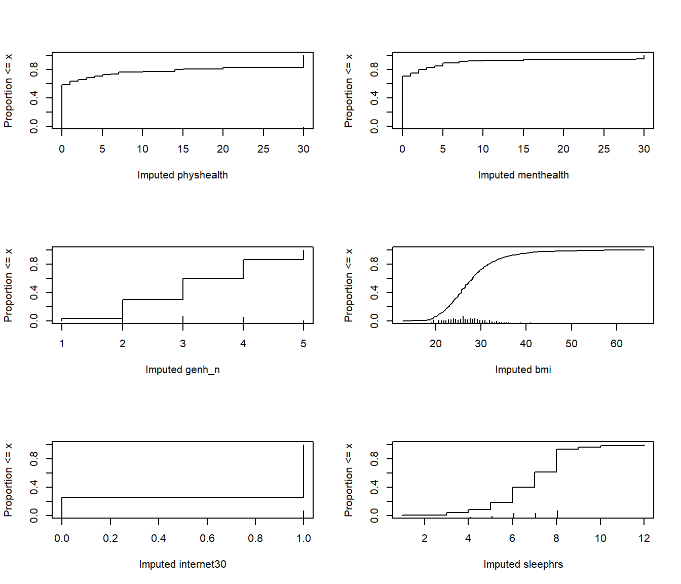
par(mfrow = c(1,1))From these cumulative distribution functions, we can see that, for example,
- we imputed
bmivalues mostly between 20 and 35, with a few values below 20 or above 40. - most of our imputed
sleephrswere between 5 and 10 - we imputed 1 for
internet30for about 70% of the subjects, and 0 for the other 30%.
This predictive mean matching method never imputes a value for a variable that does not already exist in the data.
14.11 Combining the Imputation and Outcome Models
So, now we have an imputation model, called imp_fit. and two outcome models: m1 and m2. What do we do with them?
14.11.1 Model 1 with Multiple Imputation
To build the m1_imp multiple imputation fit for model m1, we use the fit.mult.impute command, and specify the model, the fitter (here, lrm), the imputation model (xtrans = imp_fit) and the data set prior to imputation (smartcle_imp0).
m1_imp <- fit.mult.impute(exerany ~
            internet30 * catg(genh_n) + bmi * female +
            physhealth + menthealth + sleephrs,
            fitter = lrm, xtrans = imp_fit,
            data = smartcle_imp0, x = TRUE, y = TRUE)
Variance Inflation Factors Due to Imputation:

            Intercept            internet30              genh_n=2
                 1.03                  1.00                  1.01
             genh_n=3              genh_n=4              genh_n=5
                 1.00                  1.01                  1.02
                  bmi                female            physhealth
                 1.06                  1.08                  1.05
           menthealth              sleephrs internet30 * genh_n=2
                 1.01                  1.02                  1.01
internet30 * genh_n=3 internet30 * genh_n=4 internet30 * genh_n=5
                 1.00                  1.01                  1.03
         bmi * female
                 1.08

Rate of Missing Information:

            Intercept            internet30              genh_n=2
                 0.03                  0.00                  0.01
             genh_n=3              genh_n=4              genh_n=5
                 0.00                  0.01                  0.02
                  bmi                female            physhealth
                 0.05                  0.07                  0.04
           menthealth              sleephrs internet30 * genh_n=2
                 0.01                  0.02                  0.01
internet30 * genh_n=3 internet30 * genh_n=4 internet30 * genh_n=5
                 0.00                  0.01                  0.03
         bmi * female
                 0.08

d.f. for t-distribution for Tests of Single Coefficients:

            Intercept            internet30              genh_n=2
             21695.29            4552554.82             342982.63
             genh_n=3              genh_n=4              genh_n=5
           2393040.31             340219.46              43771.65
                  bmi                female            physhealth
              6985.80               3594.27               9984.27
           menthealth              sleephrs internet30 * genh_n=2
             87510.83              39656.28             292980.96
internet30 * genh_n=3 internet30 * genh_n=4 internet30 * genh_n=5
           6057039.66             610087.87              23370.34
         bmi * female
              3152.92

The following fit components were averaged over the 20 model fits:

  stats linear.predictors
OK. Let’s get the familiar description of an lrm model, after this multiple imputation.
m1_impLogistic Regression Model
fit.mult.impute(formula = exerany ~ internet30 * catg(genh_n) +
bmi * female + physhealth + menthealth + sleephrs, fitter = lrm,
xtrans = imp_fit, data = smartcle_imp0, x = TRUE, y = TRUE)
Model Likelihood Discrimination Rank Discrim.
Ratio Test Indexes Indexes
Obs 1033 LR chi2 153.52 R2 0.207 C 0.743
0 247 d.f. 15 g 1.031 Dxy 0.487
1 786 Pr(> chi2) <0.0001 gr 2.803 gamma 0.487
max |deriv| 1e-12 gp 0.176 tau-a 0.177
Brier 0.153
Coef S.E. Wald Z Pr(>|Z|)
Intercept 3.3183 0.9782 3.39 0.0007
internet30 0.6499 0.7013 0.93 0.3540
genh_n=2 -0.4613 0.7507 -0.61 0.5389
genh_n=3 -0.9069 0.6978 -1.30 0.1937
genh_n=4 -1.3287 0.7392 -1.80 0.0722
genh_n=5 -0.9257 0.8342 -1.11 0.2671
bmi -0.0408 0.0216 -1.89 0.0588
female -0.9153 0.7786 -1.18 0.2398
physhealth -0.0234 0.0103 -2.27 0.0235
menthealth -0.0192 0.0115 -1.68 0.0934
sleephrs -0.0407 0.0496 -0.82 0.4120
internet30 * genh_n=2 0.3503 0.8117 0.43 0.6661
internet30 * genh_n=3 0.1110 0.7549 0.15 0.8832
internet30 * genh_n=4 -0.1851 0.8117 -0.23 0.8196
internet30 * genh_n=5 -1.2268 0.9748 -1.26 0.2082
bmi * female 0.0108 0.0263 0.41 0.6822
We can obtain an ANOVA plot and an AIC plot to look at the predictors:
par(mfrow = c(2,1))
plot(anova(m1_imp))
plot(anova(m1_imp), what="aic")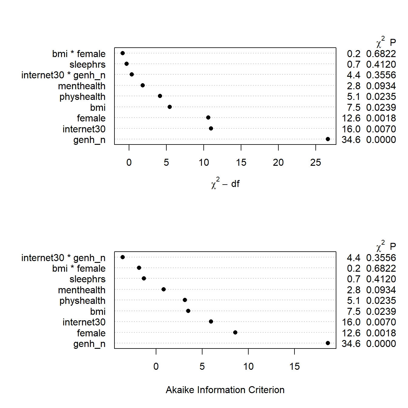
par(mfrow = c(1,1))Here’s the summary of effect sizes.
summary(m1_imp) Effects Response : exerany
Factor Low High Diff. Effect S.E. Lower 0.95 Upper 0.95
internet30 0.0 1.00 1.00 1.000300 0.411430 0.193880 1.8066000
Odds Ratio 0.0 1.00 1.00 2.719000 NA 1.214000 6.0899000
bmi 23.7 30.53 6.83 -0.279000 0.147670 -0.568430 0.0104310
Odds Ratio 23.7 30.53 6.83 0.756540 NA 0.566410 1.0105000
female 0.0 1.00 1.00 -0.628260 0.181140 -0.983290 -0.2732400
Odds Ratio 0.0 1.00 1.00 0.533520 NA 0.374080 0.7609100
physhealth 0.0 2.00 2.00 -0.046783 0.020654 -0.087264 -0.0063023
Odds Ratio 0.0 2.00 2.00 0.954290 NA 0.916440 0.9937200
menthealth 0.0 2.00 2.00 -0.038477 0.022932 -0.083422 0.0064689
Odds Ratio 0.0 2.00 2.00 0.962250 NA 0.919960 1.0065000
sleephrs 6.0 8.00 2.00 -0.081454 0.099287 -0.276050 0.1131500
Odds Ratio 6.0 8.00 2.00 0.921770 NA 0.758770 1.1198000
genh_n - 1:2 2.0 1.00 NA 0.461310 0.750680 -1.010000 1.9326000
Odds Ratio 2.0 1.00 NA 1.586200 NA 0.364220 6.9076000
genh_n - 3:2 2.0 3.00 NA -0.445620 0.442710 -1.313300 0.4220800
Odds Ratio 2.0 3.00 NA 0.640430 NA 0.268930 1.5251000
genh_n - 4:2 2.0 4.00 NA -0.867380 0.500240 -1.847800 0.1130700
Odds Ratio 2.0 4.00 NA 0.420050 NA 0.157580 1.1197000
genh_n - 5:2 2.0 5.00 NA -0.464420 0.626480 -1.692300 0.7634700
Odds Ratio 2.0 5.00 NA 0.628500 NA 0.184090 2.1457000
Adjusted to: internet30=0 genh_n=2 bmi=26.68 female=0 plot(summary(m1_imp))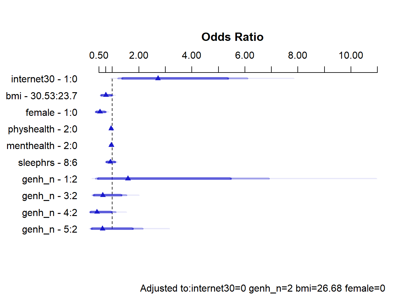
And here is the nomogram.
plot(nomogram(m1_imp, fun = plogis))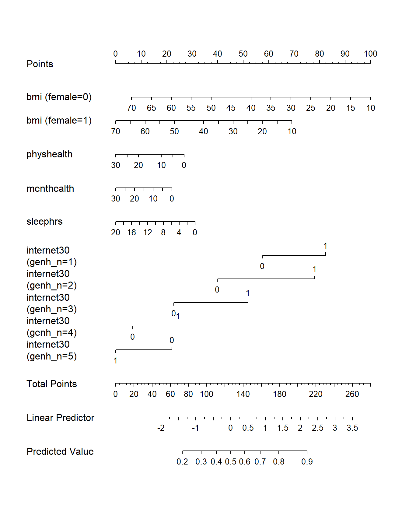
Here are the descriptive model plots, on the original probability scale for our exerany outcome:
ggplot(Predict(m1_imp), fun = plogis)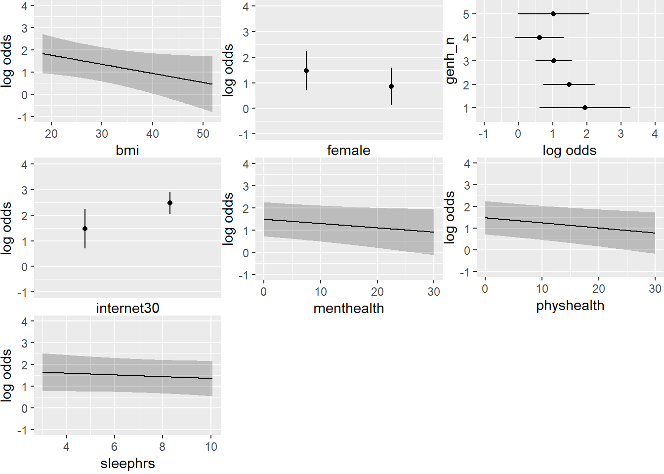
We can still do things like validate the summary statistics, too.
validate(m1_imp) index.orig training test optimism index.corrected n
Dxy 0.4889 0.5155 0.4739 0.0416 0.4473 40
R2 0.2070 0.2299 0.1912 0.0388 0.1682 40
Intercept 0.0000 0.0000 0.1047 -0.1047 0.1047 40
Slope 1.0000 1.0000 0.8922 0.1078 0.8922 40
Emax 0.0000 0.0000 0.0442 0.0442 0.0442 40
D 0.1476 0.1659 0.1355 0.0304 0.1173 40
U -0.0019 -0.0019 0.0022 -0.0041 0.0022 40
Q 0.1496 0.1678 0.1333 0.0345 0.1151 40
B 0.1533 0.1499 0.1563 -0.0064 0.1597 40
g 1.0307 1.1056 0.9773 0.1283 0.9024 40
gp 0.1764 0.1851 0.1686 0.0165 0.1599 4014.11.2 Model 2 with Multiple Imputation
The same approach is used to build the m2_imp multiple imputation fit for model m2, using the fit.mult.impute command, and specifying the model, the fitter (here, lrm), the imputation model (xtrans = imp_fit) and the data set prior to imputation (smartcle_imp0).
m2_imp <- fit.mult.impute(exerany ~
            rcs(bmi, 4) + rcs(physhealth, 5) +
            female + internet30 * catg(genh_n) +
            catg(genh_n) %ia% physhealth + female %ia% bmi +
            menthealth + sleephrs,
            fitter = lrm, xtrans = imp_fit,
            data = smartcle_imp0, x = TRUE, y = TRUE)
Variance Inflation Factors Due to Imputation:

            Intercept                   bmi                  bmi'
                 1.07                  1.08                  1.06
                bmi''            physhealth           physhealth'
                 1.06                  1.04                  1.02
               female            internet30              genh_n=2
                 1.08                  1.00                  1.01
             genh_n=3              genh_n=4              genh_n=5
                 1.00                  1.01                  1.01
genh_n=2 * physhealth genh_n=3 * physhealth genh_n=4 * physhealth
                 1.03                  1.03                  1.02
genh_n=5 * physhealth          female * bmi            menthealth
                 1.03                  1.09                  1.01
             sleephrs internet30 * genh_n=2 internet30 * genh_n=3
                 1.03                  1.01                  1.00
internet30 * genh_n=4 internet30 * genh_n=5
                 1.01                  1.04

Rate of Missing Information:

            Intercept                   bmi                  bmi'
                 0.07                  0.07                  0.06
                bmi''            physhealth           physhealth'
                 0.06                  0.04                  0.02
               female            internet30              genh_n=2
                 0.08                  0.00                  0.01
             genh_n=3              genh_n=4              genh_n=5
                 0.00                  0.01                  0.01
genh_n=2 * physhealth genh_n=3 * physhealth genh_n=4 * physhealth
                 0.03                  0.03                  0.02
genh_n=5 * physhealth          female * bmi            menthealth
                 0.03                  0.08                  0.01
             sleephrs internet30 * genh_n=2 internet30 * genh_n=3
                 0.03                  0.01                  0.00
internet30 * genh_n=4 internet30 * genh_n=5
                 0.01                  0.04

d.f. for t-distribution for Tests of Single Coefficients:

            Intercept                   bmi                  bmi'
              4380.39               3700.10               5557.48
                bmi''            physhealth           physhealth'
              5611.05              14728.96              42868.19
               female            internet30              genh_n=2
              3252.44            3009564.42             305690.58
             genh_n=3              genh_n=4              genh_n=5
           1329373.30             318205.87             190432.29
genh_n=2 * physhealth genh_n=3 * physhealth genh_n=4 * physhealth
             21003.64              22615.76              38202.98
genh_n=5 * physhealth          female * bmi            menthealth
             21998.83               3002.51             111867.55
             sleephrs internet30 * genh_n=2 internet30 * genh_n=3
             26186.82             211617.58            2865315.54
internet30 * genh_n=4 internet30 * genh_n=5
            551890.44              10977.39

The following fit components were averaged over the 20 model fits:

  stats linear.predictors
OK. Let’s get the familiar description of an lrm model, after this multiple imputation.
m2_impLogistic Regression Model
fit.mult.impute(formula = exerany ~ rcs(bmi, 4) + rcs(physhealth,
5) + female + internet30 * catg(genh_n) + catg(genh_n) %ia%
physhealth + female %ia% bmi + menthealth + sleephrs, fitter = lrm,
xtrans = imp_fit, data = smartcle_imp0, x = TRUE, y = TRUE)
Model Likelihood Discrimination Rank Discrim.
Ratio Test Indexes Indexes
Obs 1033 LR chi2 162.26 R2 0.218 C 0.746
0 247 d.f. 22 g 1.062 Dxy 0.492
1 786 Pr(> chi2) <0.0001 gr 2.892 gamma 0.492
max |deriv| 5e-12 gp 0.180 tau-a 0.179
Brier 0.152
Coef S.E. Wald Z Pr(>|Z|)
Intercept 2.9915 1.9954 1.50 0.1338
bmi -0.0164 0.0812 -0.20 0.8397
bmi' -0.2350 0.3356 -0.70 0.4837
bmi'' 0.7236 0.9089 0.80 0.4260
physhealth 0.0261 0.0862 0.30 0.7624
physhealth' -0.2434 0.3696 -0.66 0.5102
female -0.9680 0.8140 -1.19 0.2344
internet30 0.6182 0.7059 0.88 0.3812
genh_n=2 -0.4851 0.7558 -0.64 0.5210
genh_n=3 -0.8620 0.7066 -1.22 0.2225
genh_n=4 -1.2144 0.7554 -1.61 0.1079
genh_n=5 -2.7928 1.2040 -2.32 0.0204
genh_n=2 * physhealth -0.0061 0.0803 -0.08 0.9397
genh_n=3 * physhealth -0.0325 0.0775 -0.42 0.6750
genh_n=4 * physhealth -0.0322 0.0772 -0.42 0.6766
genh_n=5 * physhealth 0.0634 0.0856 0.74 0.4591
female * bmi 0.0111 0.0272 0.41 0.6831
menthealth -0.0197 0.0117 -1.68 0.0923
sleephrs -0.0554 0.0510 -1.09 0.2774
internet30 * genh_n=2 0.3882 0.8163 0.48 0.6344
internet30 * genh_n=3 0.1368 0.7617 0.18 0.8575
internet30 * genh_n=4 -0.1712 0.8203 -0.21 0.8347
internet30 * genh_n=5 -1.4939 0.9985 -1.50 0.1346
We can obtain an ANOVA plot and an AIC plot to look at the predictors:
par(mfrow = c(2,1))
plot(anova(m2_imp))
plot(anova(m2_imp), what="aic")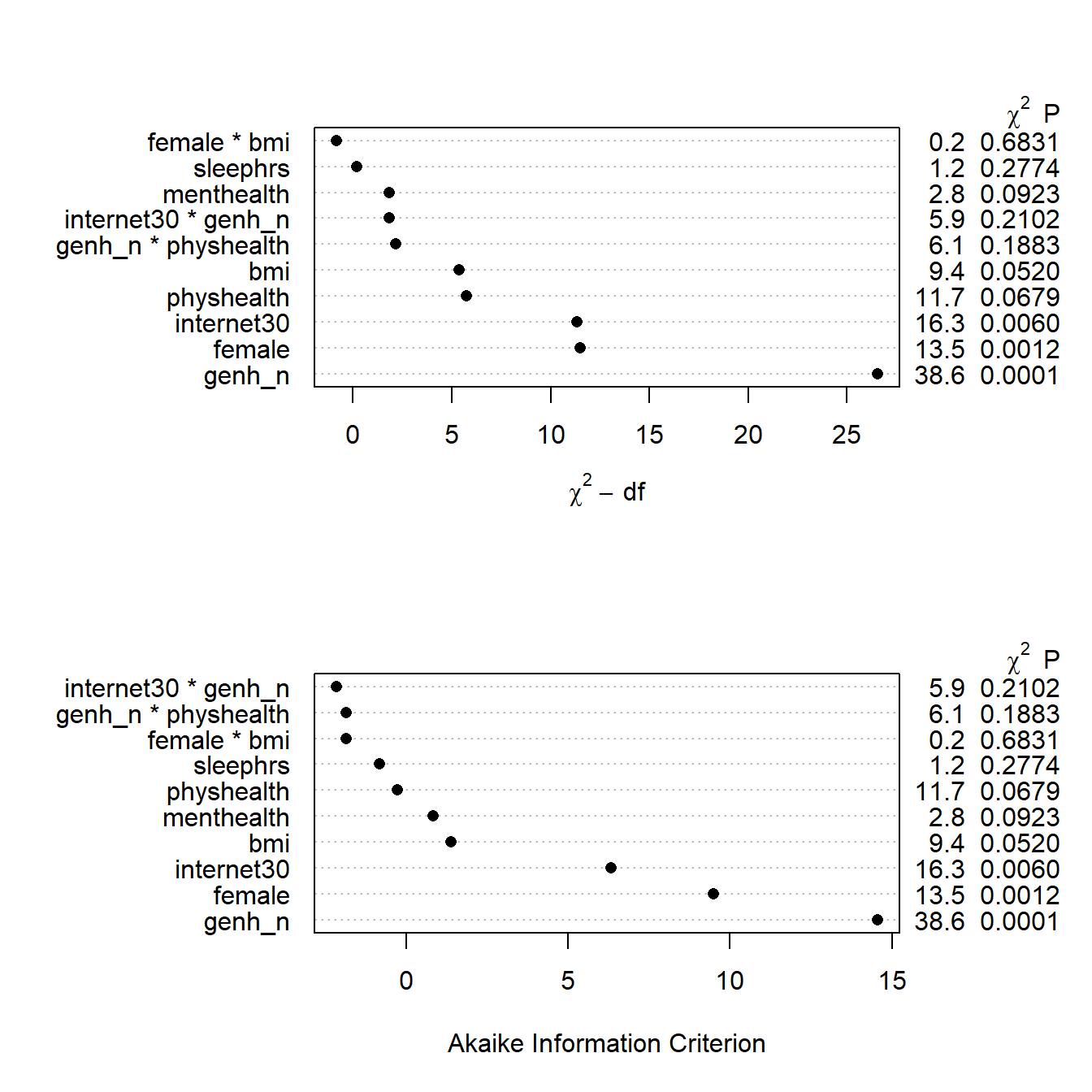
par(mfrow = c(1,1))Here’s the summary of effect sizes.
summary(m2_imp) Effects Response : exerany
Factor Low High Diff. Effect S.E. Lower 0.95 Upper 0.95
bmi 23.7 30.53 6.83 -0.498810 0.233540 -0.956540 -0.0410830
Odds Ratio 23.7 30.53 6.83 0.607250 NA 0.384220 0.9597500
physhealth 0.0 2.00 2.00 0.037808 0.100250 -0.158680 0.2343000
Odds Ratio 0.0 2.00 2.00 1.038500 NA 0.853270 1.2640000
female 0.0 1.00 1.00 -0.671780 0.189360 -1.042900 -0.3006400
Odds Ratio 0.0 1.00 1.00 0.510800 NA 0.352420 0.7403400
internet30 0.0 1.00 1.00 1.006400 0.412260 0.198370 1.8144000
Odds Ratio 0.0 1.00 1.00 2.735700 NA 1.219400 6.1374000
menthealth 0.0 2.00 2.00 -0.039395 0.023405 -0.085267 0.0064773
Odds Ratio 0.0 2.00 2.00 0.961370 NA 0.918270 1.0065000
sleephrs 6.0 8.00 2.00 -0.110820 0.102030 -0.310800 0.0891530
Odds Ratio 6.0 8.00 2.00 0.895100 NA 0.732860 1.0932000
genh_n - 1:2 2.0 1.00 NA 0.485110 0.755780 -0.996190 1.9664000
Odds Ratio 2.0 1.00 NA 1.624400 NA 0.369290 7.1450000
genh_n - 3:2 2.0 3.00 NA -0.376840 0.455990 -1.270600 0.5168800
Odds Ratio 2.0 3.00 NA 0.686030 NA 0.280670 1.6768000
genh_n - 4:2 2.0 4.00 NA -0.729310 0.526230 -1.760700 0.3020700
Odds Ratio 2.0 4.00 NA 0.482240 NA 0.171920 1.3527000
genh_n - 5:2 2.0 5.00 NA -2.307700 1.074000 -4.412600 -0.2026900
Odds Ratio 2.0 5.00 NA 0.099493 NA 0.012123 0.8165300
Adjusted to: bmi=26.68 physhealth=0 female=0 internet30=0 genh_n=2 plot(summary(m2_imp))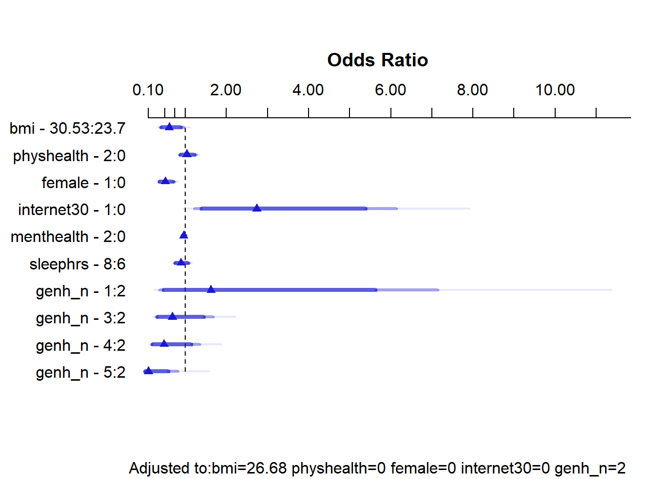
And here is the nomogram.
plot(nomogram(m2_imp, fun = plogis))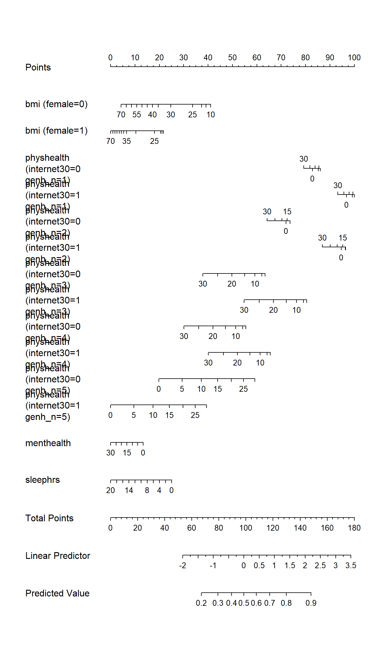
Here are the descriptive model plots, on the scale of Pr(exerany = 1):
ggplot(Predict(m2_imp), fun = plogis)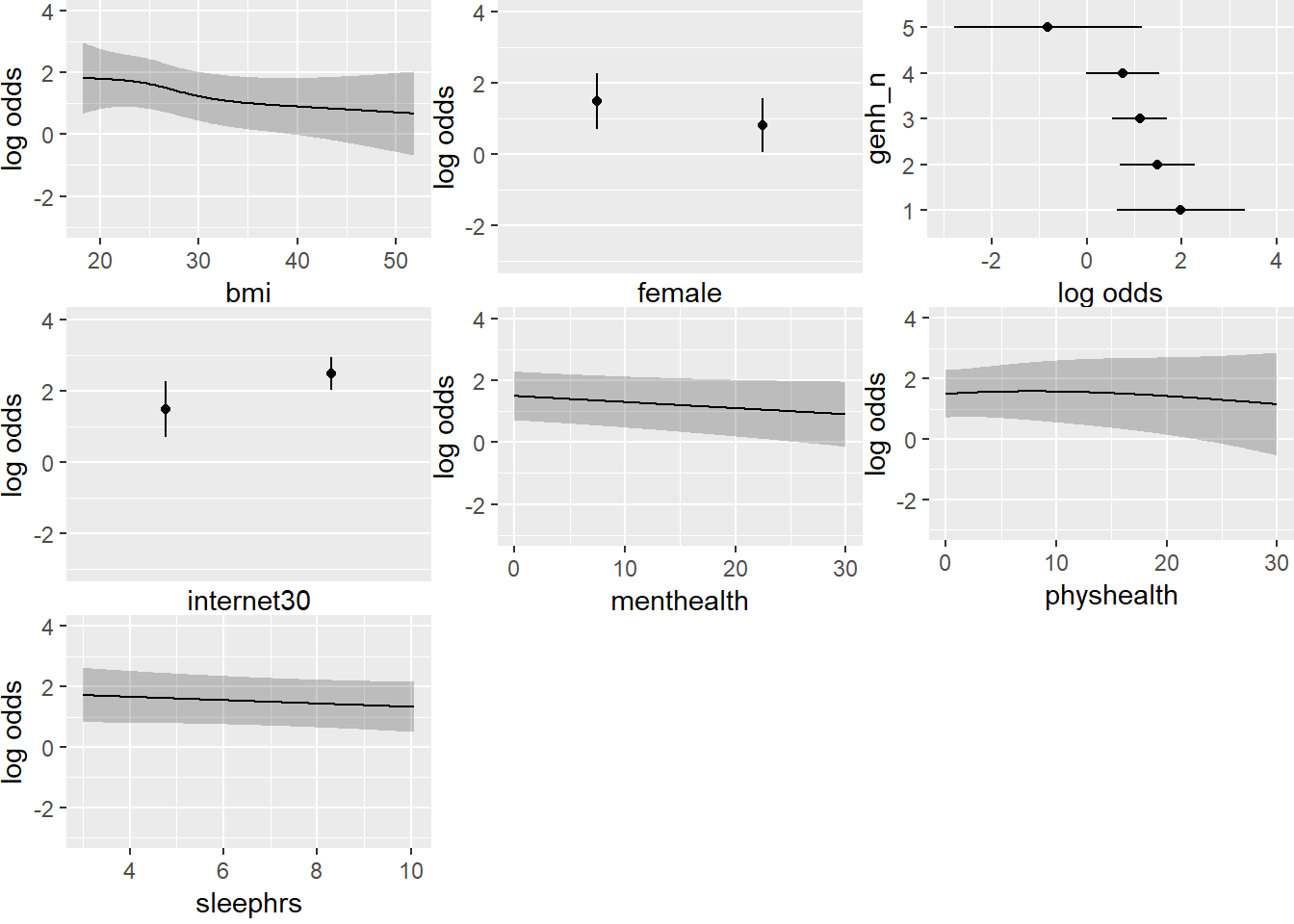
Validation of summary statistics:
validate(m2_imp) index.orig training test optimism index.corrected n
Dxy 0.4950 0.5193 0.4672 0.0521 0.4430 40
R2 0.2179 0.2461 0.1885 0.0576 0.1603 40
Intercept 0.0000 0.0000 0.1847 -0.1847 0.1847 40
Slope 1.0000 1.0000 0.8311 0.1689 0.8311 40
Emax 0.0000 0.0000 0.0759 0.0759 0.0759 40
D 0.1561 0.1787 0.1335 0.0452 0.1109 40
U -0.0019 -0.0019 0.0054 -0.0073 0.0054 40
Q 0.1580 0.1807 0.1281 0.0526 0.1055 40
B 0.1514 0.1473 0.1557 -0.0084 0.1598 40
g 1.0618 1.1583 0.9678 0.1905 0.8713 40
gp 0.1801 0.1901 0.1651 0.0250 0.1551 4014.12 Models with and without Imputation
| Model | 1 | 1 | 2 | 2 |
|---|---|---|---|---|
| Imputation | Simple | Multiple | Sim. | Mult. |
| nominal R2 | 0.204 | 0.204 | 0.214 | 0.218 |
| nominal C | 0.741 | 0.741 | 0.744 | 0.746 |
| validated R2 | 0.170 | 0.168 | 0.165 | 0.160 |
| validated C | 0.722 | 0.724 | 0.720 | 0.722 |
So, what can we conclude about the discrimination results?
100 is generally safe but time-consuming. In the old days, we used to say 5. A reasonable idea is to identify the fraction of missingness in your variable with the most missingness, and if that’s 0.10, then you should run at least 100(0.10) = 10 sets of imputations.↩