Chapter 8 Analysis of Covariance with the SMART data

In this chapter, we’ll work with the smart_cle1_sh data file again.

smart_cle1_sh <- readRDS(here("data", "smart_cle1_sh.Rds"))

8.1 A New Small Study: Predicting BMI

We’ll begin by investigating the problem of predicting bmi, at first with just three regression inputs: sex, smoke100 and physhealth, in our smart_cle1_sh data set.

• The outcome of interest is bmi.
• Inputs to the regression model are:
  • female = 1 if the subject is female, and 0 if they are male
  • smoke100 = 1 if the subject has smoked 100 cigarettes in their lifetime
  • physhealth = number of poor physical health days in past 30 (treated as quantitative)

8.1.1 Does female predict bmi well?

8.1.1.1 Graphical Assessment

ggplot(smart_cle1_sh, aes(x = female, y = bmi)) +
    geom_point()

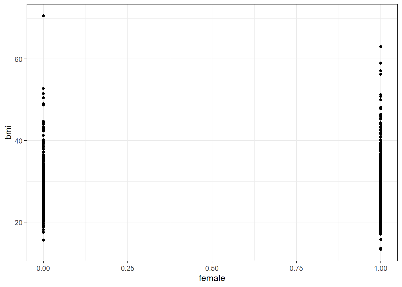
Not so helpful. We should probably specify that female is a factor, and try another plotting approach.

ggplot(smart_cle1_sh, aes(x = factor(female), y = bmi)) +
    geom_boxplot()

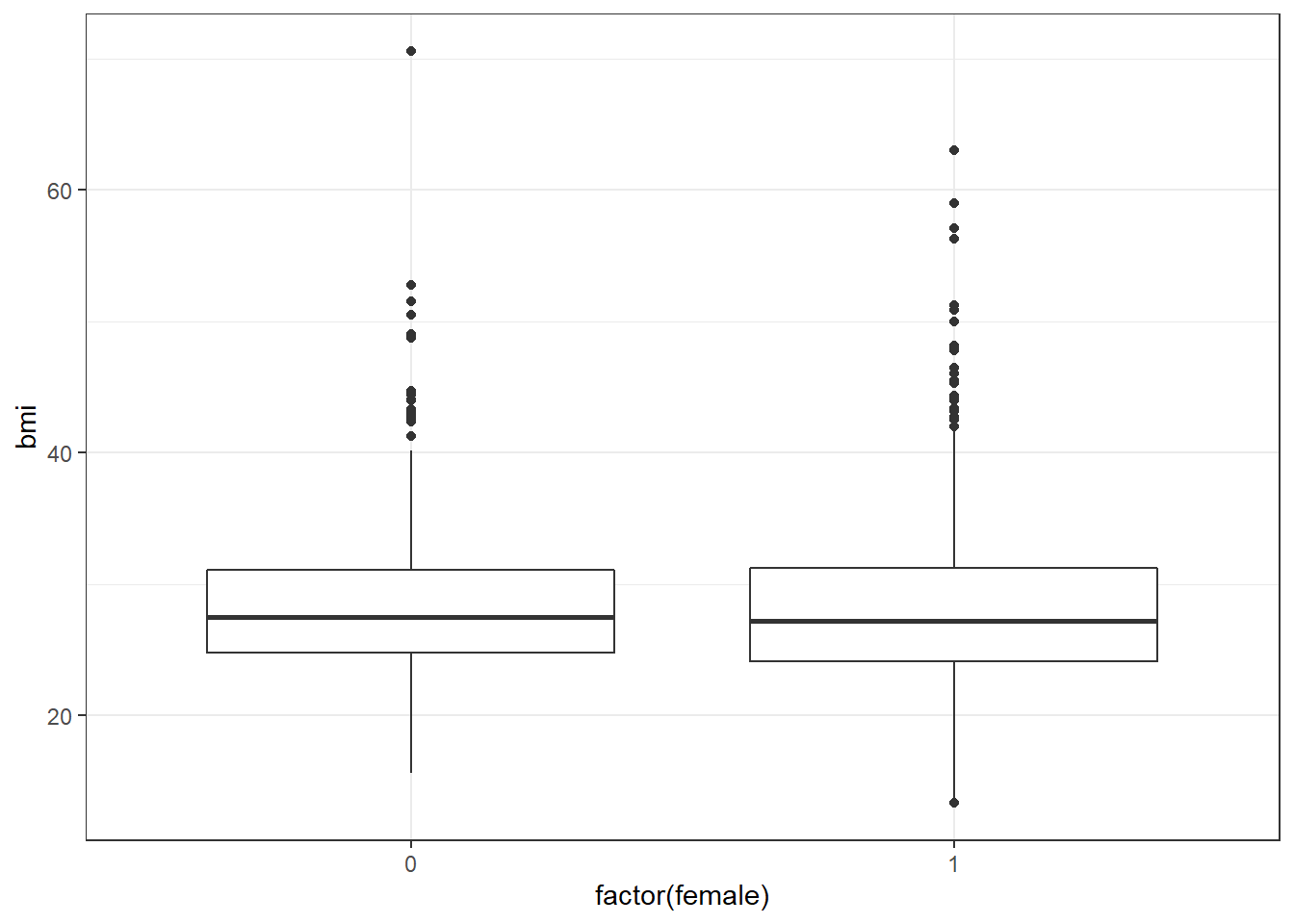
The median BMI looks a little higher for males. Let’s see if a model reflects that.

8.2 c8_m1: A simple t-test model

c8_m1 <- lm(bmi ~ female, data = smart_cle1_sh)
c8_m1

Call:
lm(formula = bmi ~ female, data = smart_cle1_sh)

Coefficients:
(Intercept)       female  
    28.5045      -0.2543  

summary(c8_m1)

Call:
lm(formula = bmi ~ female, data = smart_cle1_sh)

Residuals:
    Min      1Q  Median      3Q     Max 
-14.950  -4.065  -1.035   2.760  42.055 

Coefficients:
            Estimate Std. Error t value Pr(>|t|)    
(Intercept)  28.5045     0.2966   96.11   <2e-16 ***
female       -0.2543     0.3851   -0.66    0.509    
---
Signif. codes:  0 '***' 0.001 '**' 0.01 '*' 0.05 '.' 0.1 ' ' 1

Residual standard error: 6.368 on 1131 degrees of freedom
Multiple R-squared:  0.0003855, Adjusted R-squared:  -0.0004983 
F-statistic: 0.4362 on 1 and 1131 DF,  p-value: 0.5091

confint(c8_m1)

                2.5 %     97.5 %
(Intercept) 27.922637 29.0864336
female      -1.009911  0.5012382

The model suggests, based on these 896 subjects, that

• our best prediction for males is BMI = 28.36 kg/m², and
• our best prediction for females is BMI = 28.36 - 0.85 = 27.51 kg/m².
• the mean difference between females and males is -0.85 kg/m² in BMI
• a 95% confidence (uncertainty) interval for that mean female - male difference in BMI ranges from -1.69 to -0.01
• the model accounts for 0.4% of the variation in BMI, so that knowing the respondent’s sex does very little to reduce the size of the prediction errors as compared to an intercept only model that would predict the overall mean (regardless of sex) for all subjects.
• the model makes some enormous errors, with one subject being predicted to have a BMI 38 points lower than his/her actual BMI.

Note that this simple regression model just gives us the t-test.

t.test(bmi ~ female, var.equal = TRUE, data = smart_cle1_sh)

    Two Sample t-test

data:  bmi by female
t = 0.66046, df = 1131, p-value = 0.5091
alternative hypothesis: true difference in means is not equal to 0
95 percent confidence interval:
 -0.5012382  1.0099114
sample estimates:
mean in group 0 mean in group 1 
       28.50454        28.25020 

8.3 c8_m2: Adding another predictor (two-way ANOVA without interaction)

When we add in the information about smoke100 to our original model, we might first picture the data. We could look at separate histograms,

ggplot(smart_cle1_sh, aes(x = bmi)) +
    geom_histogram(bins = 30) +
    facet_grid(female ~ smoke100, labeller = label_both)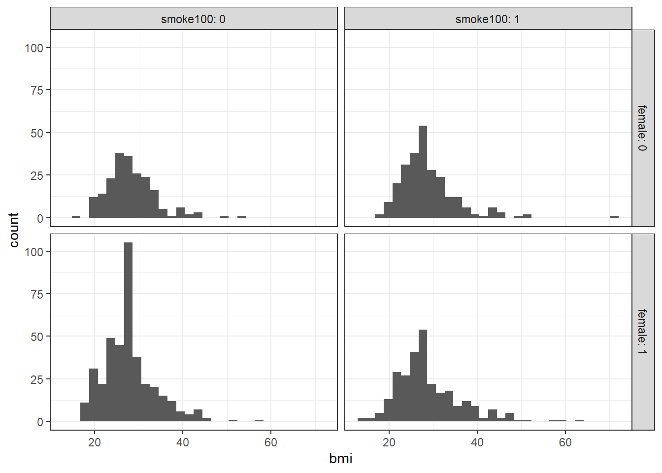

or maybe boxplots?

ggplot(smart_cle1_sh, aes(x = factor(female), y = bmi)) +
    geom_boxplot() +
    facet_wrap(~ smoke100, labeller = label_both)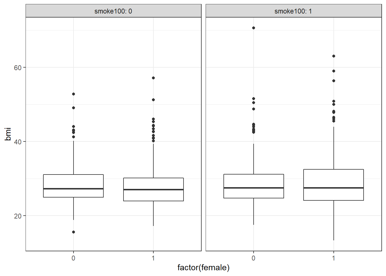

ggplot(smart_cle1_sh, aes(x = female, y = bmi))+
    geom_point(size = 3, alpha = 0.2) +
    theme_bw() +
    facet_wrap(~ smoke100, labeller = label_both)

OK. Let’s try fitting a model.

c8_m2 <- lm(bmi ~ female + smoke100, data = smart_cle1_sh)
c8_m2

Call:
lm(formula = bmi ~ female + smoke100, data = smart_cle1_sh)

Coefficients:
(Intercept)       female     smoke100  
    28.0352      -0.1440       0.8586  

This new model predicts only four predicted values:

• bmi = 28.035 if the subject is male and has not smoked 100 cigarettes (so female = 0 and smoke100 = 0)
• bmi = 28.035 - 0.144 = 27.891 if the subject is female and has not smoked 100 cigarettes (female = 1 and smoke100 = 0)
• bmi = 28.035 + 0.859 = 28.894 if the subject is male and has smoked 100 cigarettes (so female = 0 and smoke100 = 1), and, finally
• bmi = 28.035 - 0.144 + 0.859 = 28.750 if the subject is female and has smoked 100 cigarettes (so both female and smoke100 = 1).

Another way to put this is that for those who have not smoked 100 cigarettes, the model is:

• bmi = 28.035 - 0.144 female

and for those who have smoked 100 cigarettes, the model is:

• bmi = 28.894 - 0.144 female

Only the intercept of the bmi-female model changes depending on smoke100.

summary(c8_m2)

Call:
lm(formula = bmi ~ female + smoke100, data = smart_cle1_sh)

Residuals:
    Min      1Q  Median      3Q     Max 
-15.450  -3.984  -0.822   2.765  41.666 

Coefficients:
            Estimate Std. Error t value Pr(>|t|)    
(Intercept)  28.0352     0.3621  77.426   <2e-16 ***
female       -0.1440     0.3875  -0.372   0.7102    
smoke100      0.8586     0.3814   2.251   0.0246 *  
---
Signif. codes:  0 '***' 0.001 '**' 0.01 '*' 0.05 '.' 0.1 ' ' 1

Residual standard error: 6.356 on 1130 degrees of freedom
Multiple R-squared:  0.004848,  Adjusted R-squared:  0.003087 
F-statistic: 2.753 on 2 and 1130 DF,  p-value: 0.06419

confint(c8_m2)

                 2.5 %    97.5 %
(Intercept) 27.3247718 28.745657
female      -0.9043507  0.616298
smoke100     0.1102263  1.606892

The slopes of both female and smoke100 have confidence intervals that are completely below zero, indicating that both female sex and smoke100 appear to be associated with reductions in bmi.

The R² value suggests that just under 3% of the variation in bmi is accounted for by this ANOVA model.

In fact, this regression (on two binary indicator variables) is simply a two-way ANOVA model without an interaction term.

anova(c8_m2)

Analysis of Variance Table

Response: bmi
            Df Sum Sq Mean Sq F value  Pr(>F)  
female       1     18  17.687  0.4378 0.50833  
smoke100     1    205 204.733  5.0673 0.02457 *
Residuals 1130  45655  40.403                  
---
Signif. codes:  0 '***' 0.001 '**' 0.01 '*' 0.05 '.' 0.1 ' ' 1

8.4 c8_m3: Adding the interaction term (Two-way ANOVA with interaction)

Suppose we want to let the effect of female vary depending on the smoke100 status. Then we need to incorporate an interaction term in our model.

c8_m3 <- lm(bmi ~ female * smoke100, data = smart_cle1_sh)
c8_m3

Call:
lm(formula = bmi ~ female * smoke100, data = smart_cle1_sh)

Coefficients:
    (Intercept)           female         smoke100  female:smoke100  
        28.2754          -0.5126           0.4192           0.7464  

So, for example, for a male who has smoked 100 cigarettes, this model predicts

• bmi = 28.275 - 0.513 (0) + 0.419 (1) + 0.746 (0)(1) = 28.275 + 0.419 = 28.694

And for a female who has smoked 100 cigarettes, the model predicts

• bmi = 28.275 - 0.513 (1) + 0.419 (1) + 0.746 (1)(1) = 28.275 - 0.513 + 0.419 + 0.746 = 28.927

For those who have not smoked 100 cigarettes, the model is:

• bmi = 28.275 - 0.513 female

But for those who have smoked 100 cigarettes, the model is:

• bmi = (28.275 + 0.419) + (-0.513 + 0.746) female, or ,,,
• bmi = 28.694 - 0.233 female

Now, both the slope and the intercept of the bmi-female model change depending on smoke100.

summary(c8_m3)

Call:
lm(formula = bmi ~ female * smoke100, data = smart_cle1_sh)

Residuals:
    Min      1Q  Median      3Q     Max 
-15.628  -3.945  -0.833   2.745  41.865 

Coefficients:
                Estimate Std. Error t value Pr(>|t|)    
(Intercept)      28.2754     0.4397  64.308   <2e-16 ***
female           -0.5126     0.5447  -0.941    0.347    
smoke100          0.4192     0.5947   0.705    0.481    
female:smoke100   0.7464     0.7751   0.963    0.336    
---
Signif. codes:  0 '***' 0.001 '**' 0.01 '*' 0.05 '.' 0.1 ' ' 1

Residual standard error: 6.357 on 1129 degrees of freedom
Multiple R-squared:  0.005665,  Adjusted R-squared:  0.003023 
F-statistic: 2.144 on 3 and 1129 DF,  p-value: 0.09301

confint(c8_m3)

                     2.5 %     97.5 %
(Intercept)     27.4127045 29.1381042
female          -1.5812824  0.5560741
smoke100        -0.7476722  1.5860003
female:smoke100 -0.7743868  2.2672458

In fact, this regression (on two binary indicator variables and a product term) is simply a two-way ANOVA model with an interaction term.

anova(c8_m3)

Analysis of Variance Table

Response: bmi
                  Df Sum Sq Mean Sq F value  Pr(>F)  
female             1     18  17.687  0.4377 0.50835  
smoke100           1    205 204.733  5.0670 0.02458 *
female:smoke100    1     37  37.471  0.9274 0.33575  
Residuals       1129  45618  40.405                  
---
Signif. codes:  0 '***' 0.001 '**' 0.01 '*' 0.05 '.' 0.1 ' ' 1

The interaction term doesn’t change very much here. Its uncertainty interval includes zero, and the overall model still accounts for just under 3% of the variation in bmi.

8.5 c8_m4: Using female and physhealth in a model for bmi

ggplot(smart_cle1_sh, aes(x = physhealth, y = bmi, color = factor(female))) +
    geom_point() + 
    guides(col = FALSE) +
    geom_smooth(method = "lm", se = FALSE) +
    facet_wrap(~ female, labeller = label_both) 

`geom_smooth()` using formula 'y ~ x'

Does the difference in slopes of bmi and physhealth for males and females appear to be substantial and important?

c8_m4 <- lm(bmi ~ female * physhealth, data = smart_cle1_sh)

summary(c8_m4)

Call:
lm(formula = bmi ~ female * physhealth, data = smart_cle1_sh)

Residuals:
    Min      1Q  Median      3Q     Max 
-18.070  -3.826  -0.631   2.508  38.504 

Coefficients:
                  Estimate Std. Error t value Pr(>|t|)    
(Intercept)       27.93235    0.32199  86.750  < 2e-16 ***
female            -0.31175    0.42349  -0.736    0.462    
physhealth         0.13746    0.03278   4.194 2.96e-05 ***
female:physhealth -0.01247    0.04191  -0.297    0.766    
---
Signif. codes:  0 '***' 0.001 '**' 0.01 '*' 0.05 '.' 0.1 ' ' 1

Residual standard error: 6.262 on 1129 degrees of freedom
Multiple R-squared:  0.03499,   Adjusted R-squared:  0.03242 
F-statistic: 13.64 on 3 and 1129 DF,  p-value: 9.552e-09

Does it seem as though the addition of physhealth has improved our model substantially over a model with female alone (which, you recall, was c8_m1)?

Since the c8_m4 model contains the c8_m1 model’s predictors as a subset and the outcome is the same for each model, we consider the models nested and have some extra tools available to compare them.

• I might start by looking at the basic summaries for each model.

glance(c8_m4)

# A tibble: 1 x 11
  r.squared adj.r.squared sigma statistic p.value    df logLik   AIC   BIC
      <dbl>         <dbl> <dbl>     <dbl>   <dbl> <int>  <dbl> <dbl> <dbl>
1    0.0350        0.0324  6.26      13.6 9.55e-9     4 -3684. 7378. 7403.
# ... with 2 more variables: deviance <dbl>, df.residual <int>

glance(c8_m1)

# A tibble: 1 x 11
  r.squared adj.r.squared sigma statistic p.value    df logLik   AIC   BIC
      <dbl>         <dbl> <dbl>     <dbl>   <dbl> <int>  <dbl> <dbl> <dbl>
1  0.000386     -0.000498  6.37     0.436   0.509     2 -3704. 7414. 7429.
# ... with 2 more variables: deviance <dbl>, df.residual <int>

• The R² is much larger for the model with physhealth, but still very tiny.
• Smaller AIC and smaller BIC statistics are more desirable. Here, there’s little to choose from, so c8_m4 looks better, too.
• We might also consider a significance test by looking at an ANOVA model comparison. This is only appropriate because c8_m1 is nested in c8_m4.

anova(c8_m4, c8_m1)

Analysis of Variance Table

Model 1: bmi ~ female * physhealth
Model 2: bmi ~ female
  Res.Df   RSS Df Sum of Sq     F    Pr(>F)    
1   1129 44272                                 
2   1131 45860 -2   -1587.4 20.24 2.311e-09 ***
---
Signif. codes:  0 '***' 0.001 '**' 0.01 '*' 0.05 '.' 0.1 ' ' 1

The addition of the physhealth term appears to be a statistically detectable improvement, not that that means very much.

8.6 Making Predictions with a Linear Regression Model

Recall model 4, which yields predictions for body mass index on the basis of the main effects of sex (female) and days of poor physical health (physhealth) and their interaction.

c8_m4

Call:
lm(formula = bmi ~ female * physhealth, data = smart_cle1_sh)

Coefficients:
      (Intercept)             female         physhealth  female:physhealth  
         27.93235           -0.31175            0.13746           -0.01247  

8.6.1 Fitting an Individual Prediction and 95% Prediction Interval

What do we predict for the bmi of a subject who is female and had 8 poor physical health days in the past 30?

c8_new1 <- tibble(female = 1, physhealth = 8)
predict(c8_m4, newdata = c8_new1, interval = "prediction", level = 0.95)

       fit      lwr      upr
1 28.62052 16.32379 40.91724

The predicted bmi for this new subject is shown above. The prediction interval shows the bounds of a 95% uncertainty interval for a predicted bmi for an individual female subject who has 8 days of poor physical health out of the past 30. From the predict function applied to a linear model, we can get the prediction intervals for any new data points in this manner.

8.6.2 Confidence Interval for an Average Prediction

• What do we predict for the average body mass index of a population of subjects who are female and have physhealth = 8?

predict(c8_m4, newdata = c8_new1, interval = "confidence", level = 0.95)

       fit      lwr      upr
1 28.62052 28.12282 29.11822

• How does this result compare to the prediction interval?

8.6.3 Fitting Multiple Individual Predictions to New Data

• How does our prediction change for a respondent if they instead have 7, or 9 poor physical health days? What if they are male, instead of female?

c8_new2 <- tibble(subjectid = 1001:1006, female = c(1, 1, 1, 0, 0, 0), physhealth = c(7, 8, 9, 7, 8, 9))
pred2 <- predict(c8_m4, newdata = c8_new2, interval = "prediction", level = 0.95) %>% tbl_df

result2 <- bind_cols(c8_new2, pred2)
result2

# A tibble: 6 x 6
  subjectid female physhealth   fit   lwr   upr
      <int>  <dbl>      <dbl> <dbl> <dbl> <dbl>
1      1001      1          7  28.5  16.2  40.8
2      1002      1          8  28.6  16.3  40.9
3      1003      1          9  28.7  16.4  41.0
4      1004      0          7  28.9  16.6  41.2
5      1005      0          8  29.0  16.7  41.3
6      1006      0          9  29.2  16.9  41.5

The result2 tibble contains predictions for each scenario.

• Which has a bigger impact on these predictions and prediction intervals? A one category change in female or a one hour change in physhealth?

8.7 Centering the model

Our model c8_m4 has four predictors (the constant, physhealth, female and their interaction) but just two inputs (female and physhealth.) If we center the quantitative input physhealth before building the model, we get a more interpretable interaction term.

smart_cle1_sh_c <- smart_cle1_sh %>%
    mutate(physhealth_c = physhealth - mean(physhealth))

c8_m4_c <- lm(bmi ~ female * physhealth_c, data = smart_cle1_sh_c)

summary(c8_m4_c)

Call:
lm(formula = bmi ~ female * physhealth_c, data = smart_cle1_sh_c)

Residuals:
    Min      1Q  Median      3Q     Max 
-18.070  -3.826  -0.631   2.508  38.504 

Coefficients:
                    Estimate Std. Error t value Pr(>|t|)    
(Intercept)         28.57583    0.29215  97.812  < 2e-16 ***
female              -0.37011    0.37920  -0.976    0.329    
physhealth_c         0.13746    0.03278   4.194 2.96e-05 ***
female:physhealth_c -0.01247    0.04191  -0.297    0.766    
---
Signif. codes:  0 '***' 0.001 '**' 0.01 '*' 0.05 '.' 0.1 ' ' 1

Residual standard error: 6.262 on 1129 degrees of freedom
Multiple R-squared:  0.03499,   Adjusted R-squared:  0.03242 
F-statistic: 13.64 on 3 and 1129 DF,  p-value: 9.552e-09

What has changed as compared to the original c8_m4?

• Our original model was bmi = 27.93 - 0.31 female + 0.14 physhealth - 0.01 female x physhealth
• Our new model is bmi = 28.58 - 0.37 female + 0.14 centered physhealth - 0.01 female x centered physhealth.

So our new model on centered data is:

• 28.58 + 0.14 centered physhealth_c for male subjects, and
• (28.58 - 0.37) + (0.14 - 0.01) centered physhealth_c, or 28.21 - 0.13 centered physhealth_c for female subjects.

In our new (centered physhealth_c) model,

• the main effect of female now corresponds to a predictive difference (female - male) in bmi with physhealth at its mean value, 4.68 days,
• the intercept term is now the predicted bmi for a male respondent with an average physhealth, and
• the product term corresponds to the change in the slope of centered physhealth_c on bmi for a female rather than a male subject, while
• the residual standard deviation and the R-squared values remain unchanged from the model before centering.

8.7.1 Plot of Model 4 on Centered physhealth: c8_m4_c

ggplot(smart_cle1_sh_c, aes(x = physhealth_c, y = bmi, group = female, col = factor(female))) +
    geom_point(alpha = 0.5, size = 2) +
    geom_smooth(method = "lm", se = FALSE) +
    guides(color = FALSE) +
    labs(x = "Poor Physical Health Days, centered", y = "Body Mass Index",
         title = "Model `c8_m4` on centered data") +
    facet_wrap(~ female, labeller = label_both)

`geom_smooth()` using formula 'y ~ x'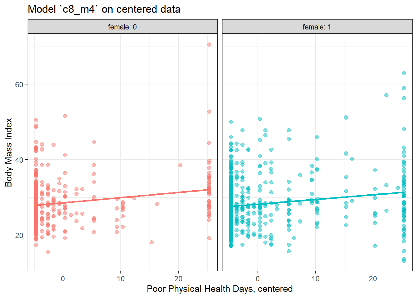

8.8 Rescaling an input by subtracting the mean and dividing by 2 standard deviations

Centering helped us interpret the main effects in the regression, but it still leaves a scaling problem.

• The female coefficient estimate is much larger than that of physhealth, but this is misleading, considering that we are comparing the complete change in one variable (sex = female or not) to a 1-day change in physhealth.
• Gelman and Hill (2007) recommend all continuous predictors be scaled by dividing by 2 standard deviations, so that:
  • a 1-unit change in the rescaled predictor corresponds to a change from 1 standard deviation below the mean, to 1 standard deviation above.
  • an unscaled binary (1/0) predictor with 50% probability of occurring will be exactly comparable to a rescaled continuous predictor done in this way.

smart_cle1_sh_rescale <- smart_cle1_sh %>%
    mutate(physhealth_z = (physhealth - mean(physhealth))/(2*sd(physhealth)))

8.8.1 Refitting model c8_m4 to the rescaled data

c8_m4_z <- lm(bmi ~ female * physhealth_z, data = smart_cle1_sh_rescale)

summary(c8_m4_z)

Call:
lm(formula = bmi ~ female * physhealth_z, data = smart_cle1_sh_rescale)

Residuals:
    Min      1Q  Median      3Q     Max 
-18.070  -3.826  -0.631   2.508  38.504 

Coefficients:
                    Estimate Std. Error t value Pr(>|t|)    
(Intercept)          28.5758     0.2921  97.812  < 2e-16 ***
female               -0.3701     0.3792  -0.976    0.329    
physhealth_z          2.5074     0.5979   4.194 2.96e-05 ***
female:physhealth_z  -0.2274     0.7646  -0.297    0.766    
---
Signif. codes:  0 '***' 0.001 '**' 0.01 '*' 0.05 '.' 0.1 ' ' 1

Residual standard error: 6.262 on 1129 degrees of freedom
Multiple R-squared:  0.03499,   Adjusted R-squared:  0.03242 
F-statistic: 13.64 on 3 and 1129 DF,  p-value: 9.552e-09

8.8.2 Interpreting the model on rescaled data

What has changed as compared to the original c8_m4?

• Our original model was bmi = 27.93 - 0.31 female + 0.14 physhealth - 0.01 female x physhealth

• Our model on centered physhealth was bmi = 28.58 - 0.37 female + 0.14 centered physhealth - 0.01 female x centered physhealth.

• Our new model on rescaled physhealth is bmi = 28.58 - 0.37 female + 2.51 rescaled physhealth_z - 0.23 female x rescaled physhealth_z.

So our rescaled model is:

• 28.58 + 2.51 rescaled physhealth_z for male subjects, and
• (28.58 - 0.37) + (2.51 - 0.23) rescaled physhealth_z, or 28.21 + 2.28 rescaled physhealth_z for female subjects.

In this new rescaled (physhealth_z) model, then,

• the main effect of female, -0.37, still corresponds to a predictive difference (female - male) in bmi with physhealth at its mean value, 4.68 days,
• the intercept term is still the predicted bmi for a male respondent with an average physhealth count, and
• the residual standard deviation and the R-squared values remain unchanged,

as before, but now we also have that:

• the coefficient of physhealth_z indicates the predictive difference in bmi associated with a change in physhealth of 2 standard deviations (from one standard deviation below the mean of 4.68 to one standard deviation above 4.68.)
  • Since the standard deviation of physhealth is 9.12 (see below), this covers a massive range of potential values of physhealth from 0 all the way up to 4.68 + 2(9.12) = 22.92 days.

mosaic::favstats(~ physhealth, data = smart_cle1_sh)

 min Q1 median Q3 max     mean       sd    n missing
   0  0      0  4  30 4.681377 9.120899 1133       0

• the coefficient of the product term (-0.23) corresponds to the change in the coefficient of physhealth_z for females as compared to males.

8.8.3 Plot of model on rescaled data

ggplot(smart_cle1_sh_rescale, aes(x = physhealth_z, y = bmi, 
                              group = female, col = factor(female))) +
    geom_point(alpha = 0.5) +
    geom_smooth(method = "lm", se = FALSE, size = 1.5) +
    scale_color_discrete(name = "Is subject female?") +
    labs(x = "Poor Physical Health Days, standardized (2 sd)", y = "Body Mass Index",
         title = "Model `c8_m4_z` on rescaled data") 

`geom_smooth()` using formula 'y ~ x'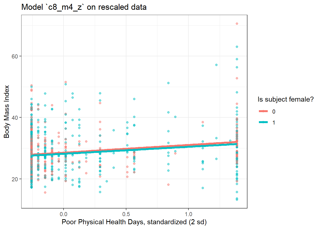

There’s very little difference here.

8.9 c8_m5: What if we add more variables?

We can boost our R² a bit, to nearly 5%, by adding in two new variables, related to whether or not the subject (in the past 30 days) used the internet, and the average number of alcoholic drinks per week consumed by ths subject.

c8_m5 <- lm(bmi ~ female + smoke100 + physhealth + internet30 + drinks_wk,
         data = smart_cle1_sh)
summary(c8_m5)

Call:
lm(formula = bmi ~ female + smoke100 + physhealth + internet30 + 
    drinks_wk, data = smart_cle1_sh)

Residuals:
    Min      1Q  Median      3Q     Max 
-18.368  -3.847  -0.659   2.523  38.035 

Coefficients:
            Estimate Std. Error t value Pr(>|t|)    
(Intercept) 27.53666    0.56081  49.101  < 2e-16 ***
female      -0.44269    0.38513  -1.149  0.25061    
smoke100     0.82917    0.37742   2.197  0.02823 *  
physhealth   0.12483    0.02074   6.019 2.38e-09 ***
internet30   0.43732    0.48835   0.896  0.37070    
drinks_wk   -0.10183    0.03352  -3.038  0.00244 ** 
---
Signif. codes:  0 '***' 0.001 '**' 0.01 '*' 0.05 '.' 0.1 ' ' 1

Residual standard error: 6.232 on 1127 degrees of freedom
Multiple R-squared:  0.04594,   Adjusted R-squared:  0.0417 
F-statistic: 10.85 on 5 and 1127 DF,  p-value: 3.26e-10

1. Here’s the ANOVA for this model. What can we study with this?

anova(c8_m5)

Analysis of Variance Table

Response: bmi
             Df Sum Sq Mean Sq F value    Pr(>F)    
female        1     18   17.69  0.4554  0.499914    
smoke100      1    205  204.73  5.2715  0.021860 *  
physhealth    1   1512 1512.41 38.9420 6.169e-10 ***
internet30    1     14   14.16  0.3646  0.546072    
drinks_wk     1    358  358.40  9.2281  0.002438 ** 
Residuals  1127  43770   38.84                      
---
Signif. codes:  0 '***' 0.001 '**' 0.01 '*' 0.05 '.' 0.1 ' ' 1

2. Consider the revised output below. Now what can we study?

anova(lm(bmi ~ smoke100 + internet30 + drinks_wk + female + physhealth,
         data = smart_cle1_sh))

Analysis of Variance Table

Response: bmi
             Df Sum Sq Mean Sq F value    Pr(>F)    
smoke100      1    217  216.84  5.5832 0.0183025 *  
internet30    1      8    8.20  0.2113 0.6458692    
drinks_wk     1    442  442.15 11.3846 0.0007658 ***
female        1     33   33.40  0.8600 0.3539334    
physhealth    1   1407 1406.80 36.2226 2.377e-09 ***
Residuals  1127  43770   38.84                      
---
Signif. codes:  0 '***' 0.001 '**' 0.01 '*' 0.05 '.' 0.1 ' ' 1

3. What does the output below let us conclude?

anova(lm(bmi ~ smoke100 + internet30 + drinks_wk + female + physhealth, 
         data = smart_cle1_sh),
      lm(bmi ~ smoke100 + female + drinks_wk, 
         data = smart_cle1_sh))

Analysis of Variance Table

Model 1: bmi ~ smoke100 + internet30 + drinks_wk + female + physhealth
Model 2: bmi ~ smoke100 + female + drinks_wk
  Res.Df   RSS Df Sum of Sq      F    Pr(>F)    
1   1127 43770                                  
2   1129 45177 -2   -1407.1 18.116 1.805e-08 ***
---
Signif. codes:  0 '***' 0.001 '**' 0.01 '*' 0.05 '.' 0.1 ' ' 1

4. What does it mean for the models to be “nested”?

8.10 c8_m6: Would adding self-reported health help?

And we can do even a bit better than that by adding in a multi-categorical measure: self-reported general health.

c8_m6 <- lm(bmi ~ female + smoke100 + physhealth + internet30 + drinks_wk + genhealth,
         data = smart_cle1_sh)
summary(c8_m6)

Call:
lm(formula = bmi ~ female + smoke100 + physhealth + internet30 + 
    drinks_wk + genhealth, data = smart_cle1_sh)

Residuals:
    Min      1Q  Median      3Q     Max 
-19.224  -3.657  -0.739   2.659  36.798 

Coefficients:
                    Estimate Std. Error t value Pr(>|t|)    
(Intercept)         25.22373    0.71117  35.468  < 2e-16 ***
female              -0.32958    0.37673  -0.875   0.3818    
smoke100             0.46176    0.37220   1.241   0.2150    
physhealth           0.04381    0.02507   1.748   0.0808 .  
internet30           0.92642    0.48280   1.919   0.0553 .  
drinks_wk           -0.07704    0.03295  -2.338   0.0195 *  
genhealth2_VeryGood  1.20790    0.56847   2.125   0.0338 *  
genhealth3_Good      3.22491    0.58017   5.559 3.40e-08 ***
genhealth4_Fair      4.13706    0.73295   5.644 2.10e-08 ***
genhealth5_Poor      5.85381    1.09269   5.357 1.02e-07 ***
---
Signif. codes:  0 '***' 0.001 '**' 0.01 '*' 0.05 '.' 0.1 ' ' 1

Residual standard error: 6.09 on 1123 degrees of freedom
Multiple R-squared:  0.09206,   Adjusted R-squared:  0.08479 
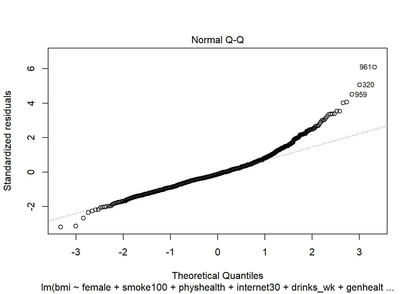
F-statistic: 12.65 on 9 and 1123 DF,  p-value: < 2.2e-16

1. If Harry and Marty have the same values of female, smoke100, physhealth, internet30 and drinks_wk, but Harry rates his health as Good, and Marty rates his as Fair, then what is the difference in the predictions? Who is predicted to have a larger BMI, and by how much?

2. What does this normal probability plot of the residuals suggest?

plot(c8_m6, which = 2)

8.11 Key Regression Assumptions for Building Effective Prediction Models

1. Validity - the data you are analyzing should map to the research question you are trying to answer.
   • The outcome should accurately reflect the phenomenon of interest.
   • The model should include all relevant predictors. (It can be difficult to decide which predictors are necessary, and what to do with predictors that have large standard errors.)
   • The model should generalize to all of the cases to which it will be applied.
   • Can the available data answer our question reliably?
2. Additivity and linearity - most important assumption of a regression model is that its deterministic component is a linear function of the predictors. We often think about transformations in this setting.
3. Independence of errors - errors from the prediction line are independent of each other
4. Equal variance of errors - if this is violated, we can more efficiently estimate parameters using weighted least squares approaches, where each point is weighted inversely proportional to its variance, but this doesn’t affect the coefficients much, if at all.
5. Normality of errors - not generally important for estimating the regression line

8.11.1 Checking Assumptions in model c8_m6

1. How does the assumption of linearity behind this model look?

plot(c8_m6, which = 1)

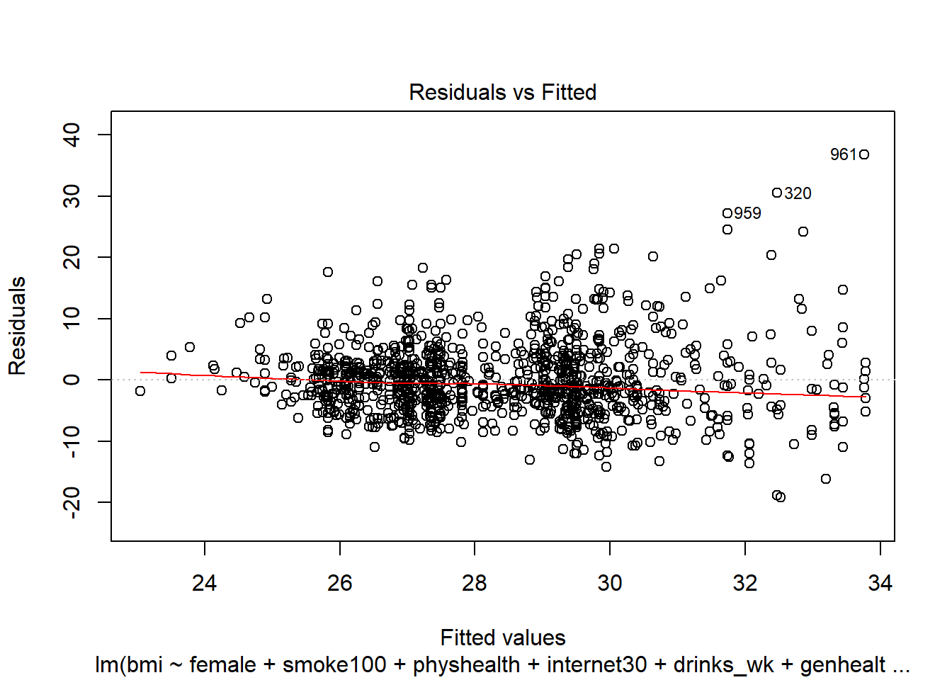
We see no strong signs of serious non-linearity here. There’s no obvious curve in the plot, for example. We may have a problem with increasing variance as we move to the right.

2. What can we conclude from the plot below?

plot(c8_m6, which = 5)

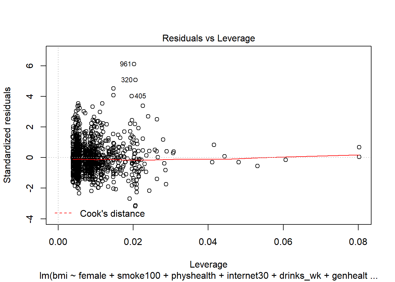
This plot can help us identify points with large standardized residuals, large leverage values, and large influence on the model (as indicated by large values of Cook’s distance.) In this case, I see no signs of any points used in the model with especially large influence, although there are some poorly fitted points (with especially large standardized residuals.)

References

Gelman, Andrew, and Jennifer Hill. 2007. Data Analysis Using Regression and Multilevel/Hierarchical Models. New York: Cambridge University Press.