Chapter 12 “Best Subsets” Variable Selection in our Prostate Cancer Study
A second approach to model selection involved fitting all possible subset models and identifying the ones that look best according to some meaningful criterion and ideally one that includes enough variables to model the response appropriately without including lots of redundant or unnecessary terms.
Here’s the set of predictors we’re considering for our modeling of lpsa, our outcome. Note that five of the eight predictors are quantitative, and the remaining three (bph, svi and gleason) are categorical. A little cleaning gives us the following results.
prost_c12 <- prost %>%
    mutate(bph = fct_relevel(factor(bph), "High", "Medium"),
           gleason = fct_relevel(factor(gleason), "6", "7"),
           svi = factor(svi))

prost_c12 %>% select(-subject, -lpsa) %>% summary()
lcavol lweight age bph svi
Min. :-1.3471 Min. :2.375 Min. :41.00 High :29 0:76
1st Qu.: 0.5128 1st Qu.:3.376 1st Qu.:60.00 Medium:25 1:21
Median : 1.4469 Median :3.623 Median :65.00 Low :43
Mean : 1.3500 Mean :3.629 Mean :63.87
3rd Qu.: 2.1270 3rd Qu.:3.876 3rd Qu.:68.00
Max. : 3.8210 Max. :4.780 Max. :79.00
lcp gleason pgg45 svi_f gleason_f bph_f
Min. :-1.3863 6 :35 Min. : 0.00 No :76 > 7: 6 Low :43
1st Qu.:-1.3863 7 :56 1st Qu.: 0.00 Yes:21 7 :56 Medium:25
Median :-0.7985 > 7: 6 Median : 15.00 6 :35 High :29
Mean :-0.1794 Mean : 24.38
3rd Qu.: 1.1787 3rd Qu.: 40.00
Max. : 2.9042 Max. :100.00
lcavol_c cavol psa
Min. :-2.69708 Min. : 0.260 Min. : 0.65
1st Qu.:-0.83719 1st Qu.: 1.670 1st Qu.: 5.65
Median : 0.09691 Median : 4.250 Median : 13.35
Mean : 0.00000 Mean : 7.001 Mean : 23.74
3rd Qu.: 0.77703 3rd Qu.: 8.390 3rd Qu.: 21.25
Max. : 2.47099 Max. :45.650 Max. :265.85 12.1 Key Summaries We’ll Use to Evaluate Potential Models (in-sample)
- Adjusted \(R^2\), which we try to maximize.
- Bayesian Information Criterion (BIC), which we also try to minimize.
- Mallows’ \(C_p\) statistic, which we will try to minimize, and which is closely related to AIC in this setting.
Choosing between AIC and BIC can be challenging.
For model selection purposes, there is no clear choice between AIC and BIC. Given a family of models, including the true model, the probability that BIC will select the correct model approaches one as the sample size n approaches infinity - thus BIC is asymptotically consistent, which AIC is not. [But, for practical purposes,] BIC often chooses models that are too simple [relative to AIC] because of its heavy penalty on complexity.
- Source: Hastie, Tibshriani, and Frideman (2001), page 208.
Several useful tools for running “all subsets” or “best subsets” regression comparisons are developed in R’s leaps package.
12.2 Using regsubsets in the leaps package
We can use the leaps package to obtain results in the prost study from looking at all possible subsets of the candidate predictors. The leaps package isn’t particularly friendly to the tidyverse. In particular, we cannot have any character variables in our predictor set. We specify our “kitchen sink” model, and apply the regsubsets function from leaps, which identifies the set of models.
To start, we’ll ask R to find the one best subset (with 1 predictor variable [in addition to the intercept], then with 2 predictors, and then with each of 3, 4, … 8 predictor variables) according to an exhaustive search without forcing any of the variables to be in or out.
- Use the
nvmaxcommand within theregsubsetsfunction to limit the number of regression inputs to a maximum. - Use the
nbestcommand to identify how many subsets you want to identify for each predictor count.
rs_mods <- regsubsets(
    lpsa ~ lcavol + lweight + age + bph +
        svi + lcp + gleason + pgg45,
    data = prost_c12, nvmax = 8, nbest = 1)

rs_summ <- summary(rs_mods)
12.2.1 Identifying the models with which and outmat
The summary of the regsubsets output provides lots of information we’ll need. To see the models selected by the system, we use:
  (Intercept) lcavol lweight   age bphMedium bphLow  svi1   lcp gleason7
1        TRUE   TRUE   FALSE FALSE     FALSE  FALSE FALSE FALSE    FALSE
2        TRUE   TRUE    TRUE FALSE     FALSE  FALSE FALSE FALSE    FALSE
3        TRUE   TRUE    TRUE FALSE     FALSE  FALSE  TRUE FALSE    FALSE
4        TRUE   TRUE    TRUE FALSE     FALSE  FALSE  TRUE FALSE     TRUE
5        TRUE   TRUE    TRUE  TRUE     FALSE   TRUE  TRUE FALSE    FALSE
6        TRUE   TRUE    TRUE  TRUE     FALSE   TRUE  TRUE FALSE     TRUE
7        TRUE   TRUE    TRUE  TRUE     FALSE   TRUE  TRUE  TRUE     TRUE
8        TRUE   TRUE    TRUE  TRUE     FALSE   TRUE  TRUE  TRUE     TRUE
  gleason> 7 pgg45
1      FALSE FALSE
2      FALSE FALSE
3      FALSE FALSE
4      FALSE FALSE
5      FALSE FALSE
6      FALSE FALSE
7      FALSE FALSE
8      FALSE  TRUE
Another version of this formatted for printing is:
         lcavol lweight age bphMedium bphLow svi1 lcp gleason7 gleason> 7 pgg45
1  ( 1 ) "*"    " "     " " " "       " "    " "  " " " "      " "        " "
2  ( 1 ) "*"    "*"     " " " "       " "    " "  " " " "      " "        " "
3  ( 1 ) "*"    "*"     " " " "       " "    "*"  " " " "      " "        " "
4  ( 1 ) "*"    "*"     " " " "       " "    "*"  " " "*"      " "        " "
5  ( 1 ) "*"    "*"     "*" " "       "*"    "*"  " " " "      " "        " "
6  ( 1 ) "*"    "*"     "*" " "       "*"    "*"  " " "*"      " "        " "
7  ( 1 ) "*"    "*"     "*" " "       "*"    "*"  "*" "*"      " "        " "
8  ( 1 ) "*"    "*"     "*" " "       "*"    "*"  "*" "*"      " "        "*"
So…
- the best one-predictor model used
lcavol - the best two-predictor model used
lcavolandlweight - the best three-predictor model used
lcavol,lweightandsvi - the best four-predictor model added an indicator variable for
gleason7 - the best five-predictor model added an indicator for
bphLowandageto model 3 - the best six-predictor model added a
gleason6indicator to model 5 - the best seven-predictor model added
lcpto model 6, - and the eight-input model replaced
gleason6withgleason7and also addedpgg45.
These “best subsets” models are not hierarchical. If they were, it would mean that each model was a subset of the one below it.
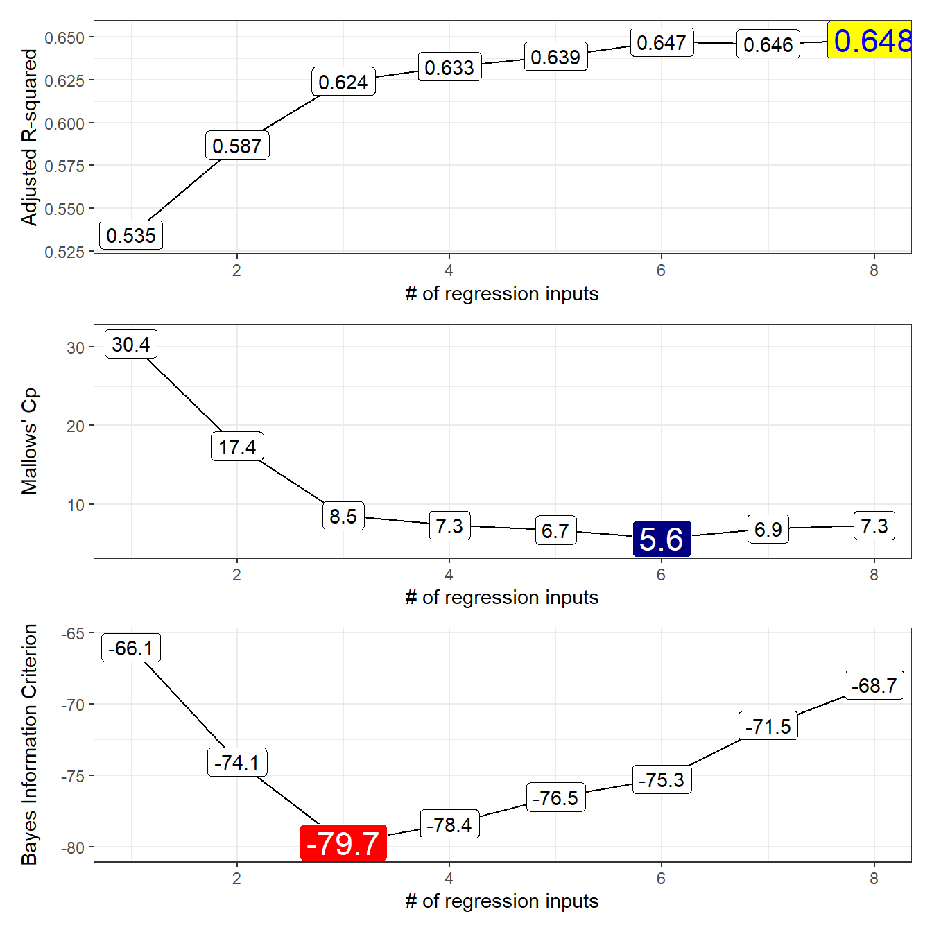
- To identify potentially attractive candidate models, we can either tabulate or plot key summaries of model fit (adjusted \(R^2\), Mallows’ \(C_p\) and BIC) using
ggplot2. I’ll show both approaches.
12.2.2 Obtaining Fit Quality Statistics
We’ll first store the summary statistics and winning models at each input count into a tibble called rs_winners. We’re doing this to facilitate plotting with ggplot2.
rs_winners <- tbl_df(rs_summ$which) %>%
    mutate(inputs = 1:(rs_mods$nvmax - 1),
           r2 = rs_summ$rsq,
           adjr2 = rs_summ$adjr2,
           cp = rs_summ$cp,
           bic = rs_summ$bic,
           rss = rs_summ$rss) %>%
    select(inputs, adjr2, cp, bic, everything())

rs_winners
# A tibble: 8 x 17
inputs adjr2 cp bic `(Intercept)` lcavol lweight age bphMedium bphLow
<int> <dbl> <dbl> <dbl> <lgl> <lgl> <lgl> <lgl> <lgl> <lgl>
1 1 0.535 30.4 -66.1 TRUE TRUE FALSE FALSE FALSE FALSE
2 2 0.587 17.4 -74.1 TRUE TRUE TRUE FALSE FALSE FALSE
3 3 0.624 8.54 -79.7 TRUE TRUE TRUE FALSE FALSE FALSE
4 4 0.633 7.31 -78.4 TRUE TRUE TRUE FALSE FALSE FALSE
5 5 0.639 6.73 -76.5 TRUE TRUE TRUE TRUE FALSE TRUE
6 6 0.647 5.64 -75.3 TRUE TRUE TRUE TRUE FALSE TRUE
7 7 0.646 6.90 -71.5 TRUE TRUE TRUE TRUE FALSE TRUE
8 8 0.648 7.34 -68.7 TRUE TRUE TRUE TRUE FALSE TRUE
# ... with 7 more variables: svi1 <lgl>, lcp <lgl>, gleason7 <lgl>, `gleason>
# 7` <lgl>, pgg45 <lgl>, r2 <dbl>, rss <dbl>12.3 Plotting the Fit Statistics
12.3.1 Plots of \(R^2\) and RMSE for each model
ggplot(rs_winners, aes(x = inputs, y = r2,
                       label = round(r2,3))) +
    geom_line() +
    geom_label() +
    geom_label(data = subset(rs_winners,
                             r2 == max(r2)),
               aes(x = inputs, y = r2,
                   label = round(r2,3)),
               fill = "black", col = "white") +
    labs(x = "# of regression inputs",
         y = "R-squared")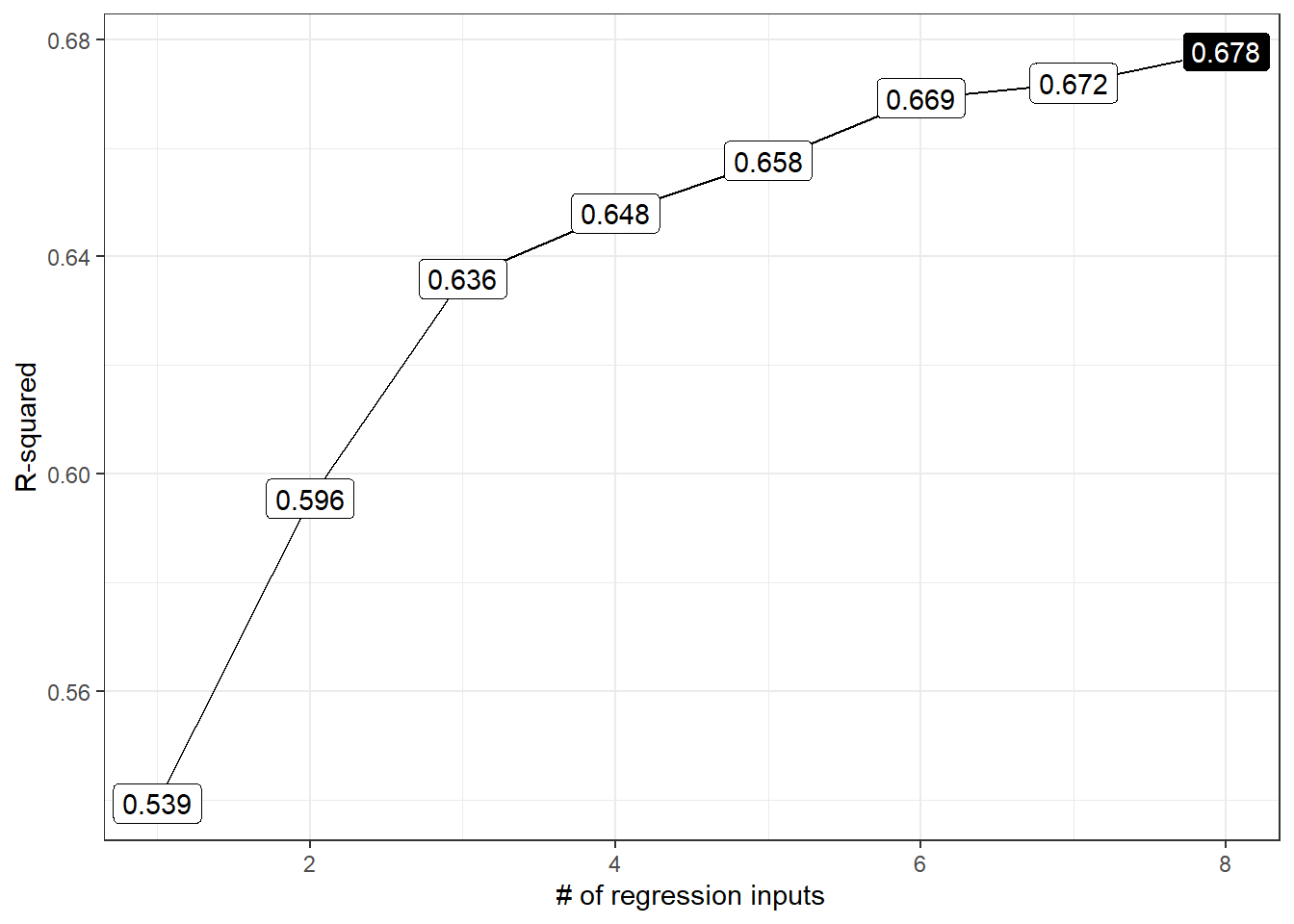
Remember that raw \(R^2\) is greedy, and will always look to select as large a set of predictors as possible. The residual sum of squares, if plotted, will have a similar problem, where the minimum RSS will always be associated with the largest model (if the models are subsets of one another.)
ggplot(rs_winners, aes(x = inputs, y = rss,
                       label = round(rss,1))) +
    geom_line() +
    geom_label() +
    geom_label(data = subset(rs_winners,
                             rss == min(rss)),
               aes(x = inputs, y = rss,
                   label = round(rss,1)),
               fill = "black", col = "white") +
    labs(x = "# of regression inputs",
         y = "Residual Sum of Squares")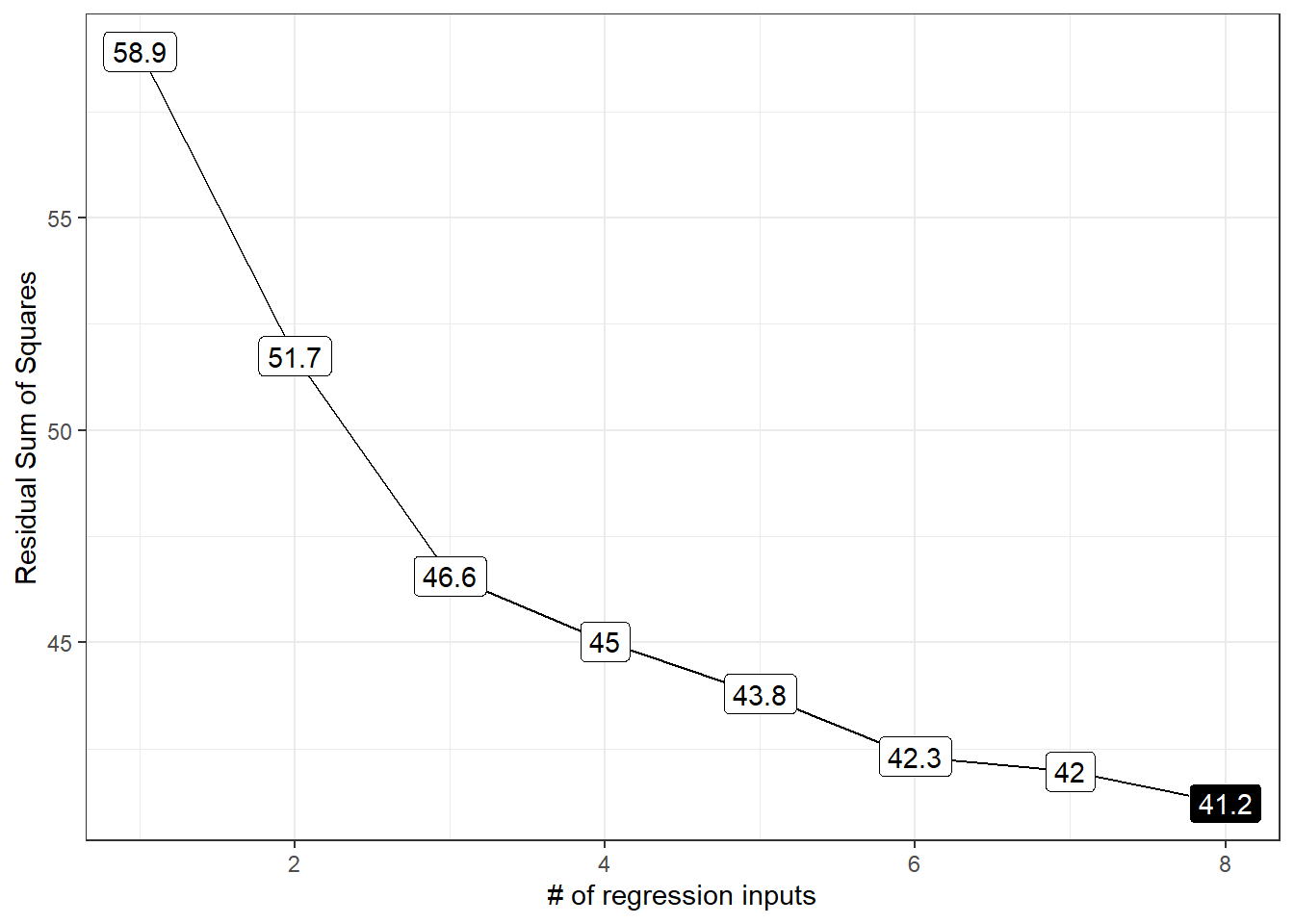
So the \(R^2\) and residual sums of squares won’t be of much help to us. Instead, we’ll focus on the three other measures we mentioned earlier.
- Adjusted \(R^2\) which we try to maximize,
- Mallows’ \(C_p\) which we try to minimize, and
- The Bayes Information Criterion (BIC) which we also try to minimize.
12.3.2 Adjusted \(R^2\) values for our subsets
p1 <- ggplot(rs_winners, aes(x = inputs, y = adjr2,
                       label = round(adjr2,3))) +
    geom_line() +
    geom_label() +
    geom_label(data = subset(rs_winners,
                             adjr2 == max(adjr2)),
               aes(x = inputs, y = adjr2,
                   label = round(adjr2,3)),
               fill = "yellow", col = "blue", size = 6) +
    scale_y_continuous(expand = expand_scale(mult = .1)) +
    labs(x = "# of regression inputs",
         y = "Adjusted R-squared")
Warning: `expand_scale()` is deprecated; use `expansion()` instead.
12.3.3 Mallows’ \(C_p\) for our subsets
The \(C_p\) statistic focuses directly on the tradeoff between bias (due to excluding important predictors from the model) and extra variance (due to including too many unimportant predictors in the model.)
If N is the sample size, and we select \(p\) regression predictors from a set of \(K\) (where \(p < K\)), then the \(C_p\) statistic is
\(C_p = \frac{SSE_p}{MSE_K} - N + 2p\)
where:
- \(SSE_p\) is the sum of squares for error (residual) in the model with \(p\) predictors
- \(MSE_K\) is the residual mean square after regression in the model with all \(K\) predictors
As it turns out, this is just measuring the particular model’s lack of fit, and then adding a penalty for the number of terms in the model (specifically \(2p - N\) is the penalty since the lack of fit is measured as \((N-p) \frac{SSE_p}{MSE_K}\).
- If a model has no meaningful lack of fit (i.e. no substantial bias) then the expected value of \(C_p\) is roughly \(p\).
- Otherwise, the expectation is \(p\) plus a positive bias term.
- In general, we want to see smaller values of \(C_p\).
p2 <- ggplot(rs_winners, aes(x = inputs, y = cp,
                       label = round(cp,1))) +
    geom_line() +
    geom_label() +
    geom_label(data = subset(rs_winners,
                             cp == min(cp)),
               aes(x = inputs, y = cp,
                   label = round(cp,1)),
               fill = "navy", col = "white", size = 6) +
    scale_y_continuous(expand = expand_scale(mult = .1)) +
    labs(x = "# of regression inputs",
         y = "Mallows' Cp")
Warning: `expand_scale()` is deprecated; use `expansion()` instead.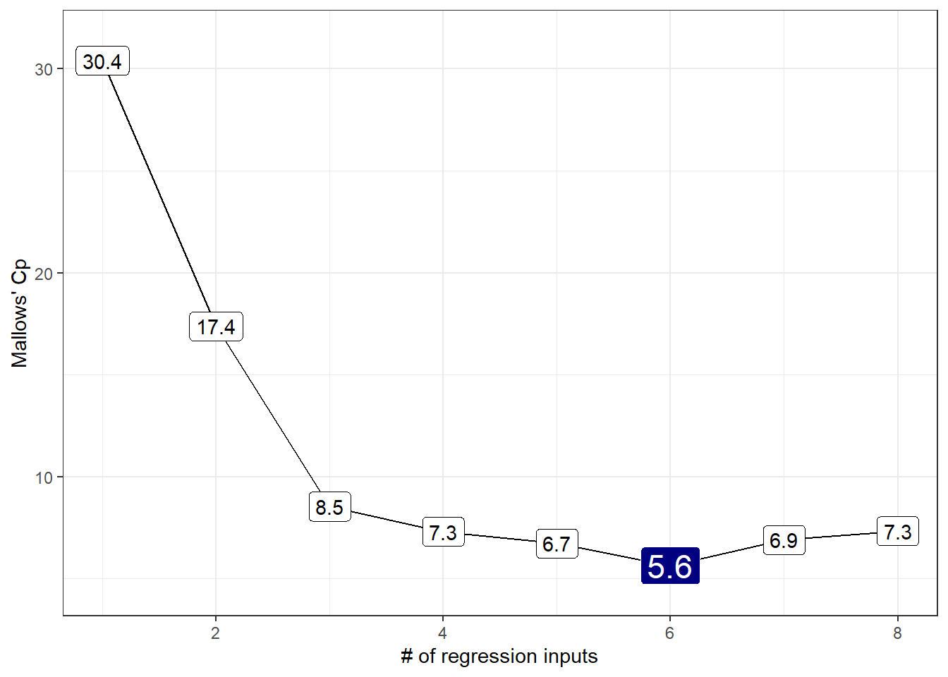
12.3.4 BIC for our subsets
We might consider several information criteria:
- the Bayesian Information Criterion, called BIC
- the Akaike Information Criterion (used by R’s default stepwise approaches,) called AIC
- a corrected version of AIC due to Hurvich and Tsai (1989), called \(AIC_c\) or
aic.c
Each of these indicates better models by getting smaller. Since the \(C_p\) and AIC results will lead to the same model, I’ll focus on plotting the BIC.
p3 <- ggplot(rs_winners, aes(x = inputs, y = bic,
                       label = round(bic, 1))) +
    geom_line() +
    geom_label() +
    geom_label(data = subset(rs_winners,
                             bic == min(bic)),
               aes(x = inputs, y = bic, label = round(bic,1)),
               fill = "red", col = "white", size = 6) +
    scale_y_continuous(expand = expand_scale(mult = .1)) +
    labs(x = "# of regression inputs",
         y = "Bayes Information Criterion")
Warning: `expand_scale()` is deprecated; use `expansion()` instead.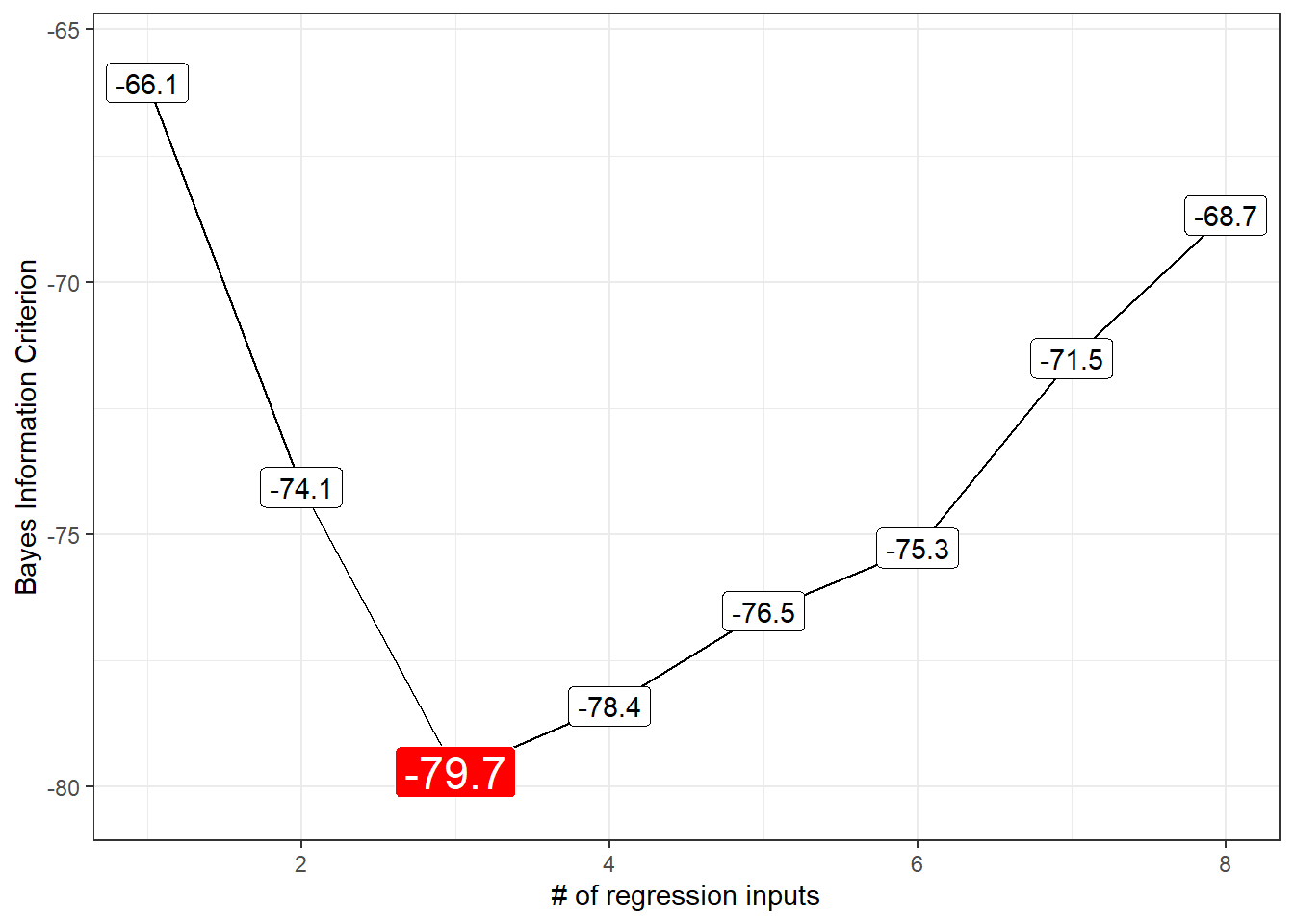
We could, if necessary, also calculate the uncorrected AIC value for each model, but we won’t make any direct use of that, because that will not provide any new information not already gathered by the \(C_p\) statistic for a linear regression model. If you wanted to find the uncorrected AIC for a given model, you can use the extractAIC function.
[1] 2.00000 -44.36603[1] 3.00000 -54.95846Note that:
- these results are fairly comparable to the bias-corrected AIC we built above, and
- the
extractAICandAICfunctions look like they give very different results, but they really don’t.
[1] 232.908[1] 222.3156But notice that the differences in AIC are the same, either way, comparing these two models:
[1] -1.00000 10.59243[1] 10.59243- AIC is only defined up to an additive constant.
- Since the difference between two models using either
AICorextractAICis the same, this doesn’t actually matter which one we use, so long as we use the same one consistently.
12.3.5 My Usual Presentation
Usually, I just plot the three useful things (adjusted \(R^2\), \(C_p\) and \(BIC\)) when I’m working with best subsets.
12.4 Which Subsets Look Best? (Tabulation)
# A tibble: 1 x 3
  AdjR2    Cp   BIC
  <int> <int> <int>
1     8     6     3
Our candidate models appear to be models 3 (minimizes BIC), 6 (minimizes \(C_p\)) and 7 (maximizes adjusted \(R^2\)).
12.4.1 Print the Coefficients of the Candidate Models
Model 3, minimizing BIC, uses lcavol, lweight and svi.
(Intercept)      lcavol     lweight        svi1
 -0.7771566   0.5258519   0.6617699   0.6656666
Model 6, minimizing \(C_p\), uses lcavol, lweight and svi, to which it adds age, and two indicator variables related to our multicategorical variables, specifically, one for bph = Low and one for gleason = 6.
(Intercept)      lcavol     lweight         age      bphLow        svi1
 0.55040580  0.50593865  0.64405366 -0.01968838 -0.30481429  0.63579895
   gleason7
 0.28167981
Model 7, maximizing adjusted \(R^2\), adds lcp to Model 6.
(Intercept)      lcavol     lweight         age      bphLow        svi1
 0.54404468  0.54144929  0.63430976 -0.02032453 -0.32131007  0.73619392
        lcp    gleason7
-0.06896264  0.29487501
12.4.2 Rerunning our candidate models
Note that the models are nested because model 3 is a subset of the predictors in model 6, which includes a subset of the predictors in model 7. We’ll also include an intercept-only model, and the full model containing all predictors we considered initially, just to show you what that would look like.
m.int <- lm(lpsa ~ 1, data = prost_c12)
model3 <- lm(lpsa ~ lcavol + lweight + svi, data = prost_c12)
model6 <- lm(lpsa ~ lcavol + lweight + svi + age +
                 (bph == "Low") + (gleason == "6"),
             data = prost_c12)
model7 <- lm(lpsa ~ lcavol + lweight + svi + age + lcp +
                 (bph == "Low") + (gleason == "6"),
             data = prost_c12)
m.full <- lm(lpsa ~ lcavol + lweight + svi +
              age + bph + gleason + lcp + pgg45,
             data = prost_c12)
12.5 Validation of Candidate Models
12.5.1 10-fold Cross-Validation of model3
Model 3 uses lcavol, lweight and svi to predict the lpsa outcome. Let’s do 10-fold cross-validation of this modeling approach, and calculate key summary measures of fit, specifically the \(R^2\), RMSE and MAE across the validation samples. We’ll use the tools from the caret package we’ve seen in prior work.
set.seed(43201)
train_c <- trainControl(method = "cv", number = 10)

model3_cv <- train(lpsa ~ lcavol + lweight + svi,
                   data = prost_c12, method = "lm",
                   trControl = train_c)

model3_cv
Linear Regression
97 samples
3 predictor
No pre-processing
Resampling: Cross-Validated (10 fold)
Summary of sample sizes: 88, 85, 87, 88, 88, 87, ...
Resampling results:
RMSE Rsquared MAE
0.7268315 0.6468265 0.5794489
Tuning parameter 'intercept' was held constant at a value of TRUE12.5.2 10-fold Cross-Validation of model6
As above, we’ll do 10-fold cross-validation of model6.
set.seed(43202)
train_c <- trainControl(method = "cv", number = 10)

model6_cv <- train(lpsa ~ lcavol + lweight + svi + age +
                       (bph == "Low") + (gleason == "6"),
                   data = prost_c12, method = "lm",
                   trControl = train_c)

model6_cv
Linear Regression
97 samples
6 predictor
No pre-processing
Resampling: Cross-Validated (10 fold)
Summary of sample sizes: 86, 88, 88, 88, 87, 87, ...
Resampling results:
RMSE Rsquared MAE
0.7036155 0.6759678 0.5533581
Tuning parameter 'intercept' was held constant at a value of TRUEThis shows a lower RMSE, higher R-squared and lower MAE than we saw in Model 3, so Model 6 looks like the better choice. How about in comparison to Model 7?
12.5.3 10-fold Cross-Validation of model7
As above, we’ll do 10-fold cross-validation of model7.
set.seed(43203)
train_c <- trainControl(method = "cv", number = 10)

model7_cv <- train(lpsa ~ lcavol + lweight + svi + age +
                       lcp + (bph == "Low") +
                       (gleason == "6"),
                   data = prost_c12, method = "lm",
                   trControl = train_c)

model7_cv
Linear Regression
97 samples
7 predictor
No pre-processing
Resampling: Cross-Validated (10 fold)
Summary of sample sizes: 88, 87, 86, 89, 88, 86, ...
Resampling results:
RMSE Rsquared MAE
0.6824712 0.6903994 0.5337871
Tuning parameter 'intercept' was held constant at a value of TRUEModel 7 looks better still, with a smaller RMSE and MAE than Model 6, and a higher R-squared. It looks like Model 7 shows best in our validation.
12.6 What about Interaction Terms?
Suppose we consider for a moment a much smaller and less realistic problem. We want to use best subsets to identify a model out of a set of three predictors for lpsa: specifically lcavol, age and svi, but now we also want to consider the interaction of svi with lcavol as a potential addition. Remember that svi a factor with levels 0 and 1. We could simply add a numerical product term to our model, as follows.
prost_c12 <- prost_c12 %>%
    mutate(svixlcavol = as.numeric(svi) * lcavol)

rs_mod2 <- regsubsets(
    lpsa ~ lcavol + age + svi + svixlcavol,
    data = prost_c12, nvmax = 4, nbest = 1)

rs_sum2 <- summary(rs_mod2)

rs_sum2
Subset selection object
Call: regsubsets.formula(lpsa ~ lcavol + age + svi + svixlcavol, data = prost_c12,
nvmax = 4, nbest = 1)
4 Variables (and intercept)
Forced in Forced out
lcavol FALSE FALSE
age FALSE FALSE
svi1 FALSE FALSE
svixlcavol FALSE FALSE
1 subsets of each size up to 4
Selection Algorithm: exhaustive
lcavol age svi1 svixlcavol
1 ( 1 ) " " " " " " "*"
2 ( 1 ) "*" " " "*" " "
3 ( 1 ) "*" " " "*" "*"
4 ( 1 ) "*" "*" "*" "*" In this case, best subsets identifies the interaction term as an attractive predictor at the very beginning, before it included the main effects that are associated with it. That’s a problem.
To resolve this, we could either:
- Consider interaction terms outside of best subsets, and only after the selection of main effects.
- Use another approach to deal with variable selection for interaction terms.
Best subsets is a very limited tool. While it’s a better choice for some problems that a stepwise regression, it suffers from some of the same problems, primarily because the resulting models are too optimistic about their measures of fit quality.
Some other tools, including ridge regression, the lasso and elastic net approaches, are sometimes more appealing.
You may be wondering if there is a “best subsets” approach which can be applied to generalized linear models. There is, in fact, a bestglm package in R which can be helpful.
But, for now, it’s time to move away from model selection and on to the very important consideration of non-linearity in the predictors.
References
Hastie, Trevor, Robert Tibshriani, and Jerome H. Frideman. 2001. The Elements of Statistical Learning. New York: Springer.
Hurvich, Clifford M., and Chih-Ling Tsai. 1989. “Regression and Time Series Model Selection in Small Samples.” Biometrika 76: 297–307. https://www.stat.berkeley.edu/~binyu/summer08/Hurvich.AICc.pdf.