33  NEW!! Bayes and a Linear Model

Almost all of this material is based on

• https://mc-stan.org/rstanarm/articles/continuous.html and
• https://easystats.github.io/bayestestR/articles/bayestestR.html and
• https://easystats.github.io/bayestestR/articles/example1.html

There’s not a lot that is truly original here. That’s a summer project.

33.1 R Setup Used Here

knitr::opts_chunk$set(comment = NA)

library(broom)
library(broom.mixed)
library(gt)
library(janitor)
library(mosaic)
library(bayestestR)
library(insight)
library(rstanarm)
library(conflicted)
library(tidyverse) 

conflicts_prefer(dplyr::select, dplyr::filter, base::mean, base::range)

theme_set(theme_bw())

33.2 Return to the smalldat Example

Consider the smalldat.csv data we discussed in Chapter 22. The data includes 150 observations on 6 variables, and one of our goals was to build a model to predict total cholesterol.

smalldat <- read_csv("data/smalldat.csv", show_col_types = FALSE)

Variable	Description
subject	Subject identification code
smoker	1 = current smoker, 0 = not current smoker
totchol	total cholesterol, in mg/dl
age	age in years
sex	subject’s sex (M or F)
educ	subject’s educational attainment (4 levels)

The educ levels are: 1_Low, 2_Middle, 3_High and 4_VHigh, which stands for Very High

33.3 The Distribution of Total Cholesterol

Across the 150 observations in the smalldat data, we have the following summaries of the distribution of total cholesterol, our outcome.

favstats(~ totchol, data = smalldat)

 min     Q1 median     Q3 max   mean       sd   n missing
 150 209.25    237 265.75 332 236.78 38.76809 150       0

33.4 Fitting a Linear Model with lm() for Total Cholesterol

m1 <- lm(totchol ~ age + sex + smoker + factor(educ), data = smalldat)

glance(m1) |> select(r.squared, adj.r.squared, sigma, 
                     AIC, BIC, df, df.residual, nobs) |>
  gt() |> fmt_number(r.squared:sigma, decimals = 3)

r.squared	adj.r.squared	sigma	AIC	BIC	df	df.residual	nobs
0.078	0.039	37.998	1525.772	1549.857	6	143	150

tidy(m1, conf.int = TRUE, conf.level = 0.95) |> 
  gt() |> fmt_number(decimals = 3)

term	estimate	std.error	statistic	p.value	conf.low	conf.high
(Intercept)	167.153	21.639	7.725	0.000	124.380	209.926
age	1.248	0.379	3.296	0.001	0.500	1.996
sexM	3.153	6.515	0.484	0.629	−9.725	16.030
smoker	3.462	6.526	0.531	0.597	−9.438	16.363
factor(educ)2_Middle	11.330	7.740	1.464	0.145	−3.970	26.631
factor(educ)3_High	−2.202	9.426	−0.234	0.816	−20.834	16.431
factor(educ)4_VHigh	11.743	9.925	1.183	0.239	−7.875	31.361

33.5 Fitting a Bayesian Linear Model

Can we fit a model for the same data using a Bayesian approach?

Yes, we can, for instance using the stan_glm() function from the rstanarm package.

set.seed(43211234) # best to set a random seed first

m2 <- stan_glm(totchol ~ age + sex + smoker + factor(educ), 
               data = smalldat, refresh = 0)

Here the refresh = 0 parameter stops the machine from printing out each of the updates it does while sampling, which is not generally something I need to look at. Here’s what’s placed in the m2 object:

m2

stan_glm
 family:       gaussian [identity]
 formula:      totchol ~ age + sex + smoker + factor(educ)
 observations: 150
 predictors:   7
------
                     Median MAD_SD
(Intercept)          166.3   21.5 
age                    1.3    0.4 
sexM                   3.1    6.5 
smoker                 3.8    6.3 
factor(educ)2_Middle  11.4    7.7 
factor(educ)3_High    -2.4    9.5 
factor(educ)4_VHigh   11.7    9.9 

Auxiliary parameter(s):
      Median MAD_SD
sigma 38.1    2.4  

------
* For help interpreting the printed output see ?print.stanreg
* For info on the priors used see ?prior_summary.stanreg

• The first few lines specify the fitting process.
• Next, for each coefficient, we find the median value from the posterior distribution, and the MAD_SD value, which is an indicator of variation derived from the estimated posterior distribution of the parameters, and is used as a standard error in what follows.
• Finally, we see the estimated root mean squared error (residual standard deviation) sigma, again estimated with the median of the sigma values in the posterior distribution.

Using the summary() function provides some additional information about the parameter estimates, but mostly some convergence diagnostics for the Markov Chain Monte Carlo procedure that the rstanarm package used to build the estimates.

summary(m2)

Model Info:
 function:     stan_glm
 family:       gaussian [identity]
 formula:      totchol ~ age + sex + smoker + factor(educ)
 algorithm:    sampling
 sample:       4000 (posterior sample size)
 priors:       see help('prior_summary')
 observations: 150
 predictors:   7

Estimates:
                       mean   sd    10%   50%   90%
(Intercept)          167.0   21.8 139.6 166.3 195.3
age                    1.2    0.4   0.8   1.3   1.7
sexM                   3.1    6.7  -5.2   3.1  11.5
smoker                 3.7    6.4  -4.5   3.8  12.0
factor(educ)2_Middle  11.3    7.9   1.2  11.4  21.3
factor(educ)3_High    -2.2    9.6 -14.3  -2.4  10.2
factor(educ)4_VHigh   11.8   10.0  -1.1  11.7  24.8
sigma                 38.2    2.3  35.4  38.1  41.3

Fit Diagnostics:
           mean   sd    10%   50%   90%
mean_PPD 236.8    4.4 231.0 236.7 242.4

The mean_ppd is the sample average posterior predictive distribution of the outcome variable (for details see help('summary.stanreg')).

MCMC diagnostics
                     mcse Rhat n_eff
(Intercept)          0.4  1.0  3208 
age                  0.0  1.0  3858 
sexM                 0.1  1.0  4725 
smoker               0.1  1.0  3941 
factor(educ)2_Middle 0.1  1.0  3535 
factor(educ)3_High   0.2  1.0  3947 
factor(educ)4_VHigh  0.2  1.0  3980 
sigma                0.0  1.0  4159 
mean_PPD             0.1  1.0  4324 
log-posterior        0.0  1.0  1773 

For each parameter, mcse is Monte Carlo standard error, n_eff is a crude measure of effective sample size, and Rhat is the potential scale reduction factor on split chains (at convergence Rhat=1).

33.5.1 Extracting the Posterior

Let’s extract the coefficients of our model, using the get_parameters() function from the insight package:

posteriors <- get_parameters(m2)

head(posteriors)

  (Intercept)       age      sexM      smoker factor(educ)2_Middle
1    147.0370 1.4540875  2.104415  15.0169219           19.5402757
2    190.0645 0.9457021  6.863091 -12.4867763            8.4980822
3    136.3315 1.6844863  7.994193   9.1766741           24.8636150
4    169.9511 1.1722918  3.785779   0.5804774            6.5798777
5    141.0931 1.5370710  7.006277  12.6397405           17.0076561
6    153.6542 1.3556864 22.009667  11.4591142           -0.9136777
  factor(educ)3_High factor(educ)4_VHigh
1           5.941676            4.100910
2          -9.449067           20.836287
3           9.972711           12.456202
4          -7.890619           16.454040
5           7.221881           -9.123619
6          -4.333041            7.401950

In all, we have 4000 observations of this posterior distribution:

nrow(posteriors)

[1] 4000

Let’s visualize the posterior distribution of our parameter for age.

ggplot(posteriors, aes(x = age)) + geom_density(fill = "dodgerblue")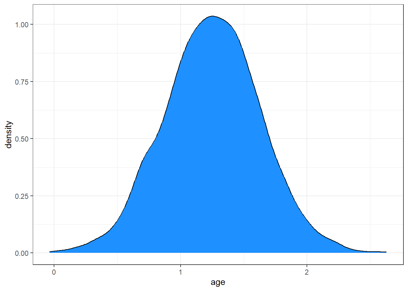

This distribution describes the probability (on the vertical axis) of various age effects (shown on the horizontal axis). Most of the distribution is between 0.5 and 2, with the peak being around 1.25.

Remember that our m1 fit with lm() had an estimated \(\beta\) for age of 1.248, so, as is often the case, there is not a lot of difference between the two models in terms of the estimates they make.

Here’s the mean and median of the age effect, across our 4000 simulations from the posterior distribution.

mean(posteriors$age)

[1] 1.249122

median(posteriors$age)

[1] 1.251402

Again, these are very close to what we obtained from least squares estimation.

Another option is to take the mode (peak) of the posterior distribution, and this is called the maximum a posteriori (MAP) estimate:

map_estimate(posteriors$age)

MAP Estimate

Parameter | MAP_Estimate
------------------------
x         |         1.26

Adding these estimates to our plot, we can see that they are all on top of each other:

ggplot(posteriors, aes(x = age)) +
  geom_density(fill = "dodgerblue") +
  # The mean in yellow
  geom_vline(xintercept = mean(posteriors$age), color = "yellow", linewidth = 1) +
  # The median in red
  geom_vline(xintercept = median(posteriors$age), color = "red", linewidth = 1) +
  # The MAP in purple
  geom_vline(xintercept = as.numeric(map_estimate(posteriors$age)), color = "purple", linewidth = 1)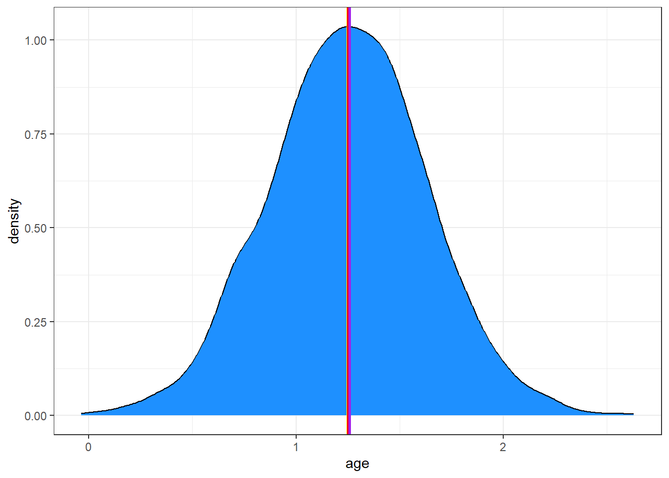

33.5.2 Describing Uncertainty

We might describe the range of estimates for the age effect.

range(posteriors$age)

[1] -0.03663079  2.63023158

Instead of showing the whole range, we usually compute the highest density interval at some percentage level, for instance a 95% credible interval which shows the range containing the 95% most probable effect values.

hdi(posteriors$age, ci = 0.95)

95% HDI: [0.50, 1.98]

So we conclude that the age effect has a 95% chance of falling within the [0.50, 1.98] range.

33.5.3 Visualizing the Coefficients and Credible Intervals

Here is a plot of the coefficients and parameters estimated in m2, along with credible intervals for their values. The inner interval (shaded region) here uses the default choice of 50%, and the outer interval (lines) uses a non-default choice of 95% (90% is the default choice here, as it turns out.) The point estimate shown here is the median of the posterior distribution, which is the default.

plot(m2, prob = 0.5, prob_outer = 0.95)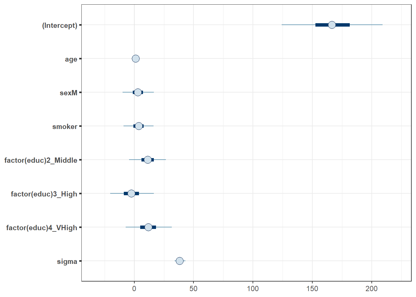

33.6 Summarizing the Posterior Distribution

A more detailed set of summaries for the posterior distribution can be obtained from the describe_posterior() function from the bayestestR package.

A brief tutorial on what is shown here is available at https://easystats.github.io/bayestestR/articles/bayestestR.html and https://easystats.github.io/bayestestR/articles/example1.html and this is the source for much of what I’ve built in this little chapter.

describe_posterior(m2) |> print_md(decimals = 3)

Summary of Posterior Distribution

Parameter	Median	95% CI	pd	ROPE	% in ROPE	Rhat	ESS
(Intercept)	166.28	[124.14, 209.25]	100%	[-3.88, 3.88]	0%	1.000	3208.00
age	1.25	[ 0.51, 1.99]	99.95%	[-3.88, 3.88]	100%	1.000	3858.00
sexM	3.07	[ -9.93, 16.46]	68.20%	[-3.88, 3.88]	42.32%	1.000	4725.00
smoker	3.75	[ -9.12, 16.17]	71.67%	[-3.88, 3.88]	41.61%	1.000	3941.00
factor(educ)2_Middle	11.39	[ -4.42, 26.57]	92.38%	[-3.88, 3.88]	14.45%	1.000	3535.00
factor(educ)3_High	-2.42	[-20.30, 16.54]	59.70%	[-3.88, 3.88]	31.45%	1.000	3947.00
factor(educ)4_VHigh	11.70	[ -7.24, 31.59]	88.00%	[-3.88, 3.88]	16.58%	0.999	3980.00

Let’s walk through all of this output.

33.6.1 Summarizing the Parameter values

For each parameter, we have:

• its estimated median across the posterior distribution
• its 95% credible interval (highest density interval of values within the posterior distribution)

as we’ve previously discussed.

33.6.2 Probability of Direction (pd) estimates.

The pd estimate helps us understand whether each effect is positive or negative. For instance, regarding age, we see the proportion of the posterior that is in the direction of the effect’s point estimate, no matter what the “size” of the effect is, will be as follows.

n_positive <- posteriors |> filter(age > 0) |> nrow()
100 * n_positive / nrow(posteriors)

[1] 99.95

So we see that the effect of age is positive with a probability of 99.95%, and this is called the probability of direction and abbreviated pd.

We can also calculate this with

p_direction(posteriors$age)

Probability of Direction

Parameter |     pd
------------------
Posterior | 99.95%

As it turns out, this pd index is usually highly correlated with the p-value from our lm() fit for age. We could almost roughly infer the corresponding p-value with a simple transformation:

pd <- 99.95
onesided_p <- 1 - pd / 100
twosided_p <- onesided_p * 2
twosided_p

[1] 0.001

This implies that the \(p\)-value for age in our lm() fit would be 0.001, and that is, in fact, what we got when we fit model m1.

The probability that each effect is in the direction shown by the point estimate is summarized in the pd column of our describe_posterior() results.

33.6.3 The ROPE estimates

Testing whether this distribution is different from 0 doesn’t make sense, as 0 is a single value (and the probability that any distribution is different from a single value is infinite). However, one way to assess significance could be to define an area around 0, which will consider as practically equivalent to zero (i.e., absence of, or a negligible, effect). This is called the Region of Practical Equivalence (ROPE).

The default (semi-objective) way of defining the ROPE is to use the tenth (1/10) of the standard deviation (SD) of the outcome variable totchol. This is sometimes considered a “negligible” effect size.

In our case, totchol has a standard deviation of 38.8, so the ROPE range is approximately (-3.88, 3.88), or somewhat more precisely:

rope_range(m2)

[1] -3.876809  3.876809

So we then compute the percentage in ROPE as the percentage of the posterior distribution that falls within this ROPE range. When most of the posterior distribution does not overlap with ROPE, we might conclude that the effect is important enough to be noted.

In our case, 100% of the age effects are in the ROPE, so that’s not really evidence of an important effect.

For smoker, though, only 42% of the effects are in the ROPE, so that’s indicative of a somewhat more substantial effect, but we’d only get really excited if a much smaller fraction, say 1%, 5% or maybe 10% were in the ROPE.

33.6.4 Convergence Diagnostics

The value of Rhat should, ideally, be 1 for each element of the model, and indicate how well the MCMC procedure converged. Generally, values of Rhat below 1.05 are good, values between 1.05 and 1.1 are OK, but values above 1.1 are too high. Here, as you can see, we don’t see any serious problems.

As for ESS, we’d like to see values of 1000 or more to ensure sufficiently stable estimates. Here, again, we’re OK.

broom.mixed::tidy(m2, conf.int = TRUE, conf.level = 0.95) |> 
  gt() |> fmt_number(decimals = 3)

term	estimate	std.error	conf.low	conf.high
(Intercept)	166.284	21.546	124.137	209.245
age	1.251	0.374	0.511	1.992
sexM	3.074	6.538	−9.929	16.461
smoker	3.753	6.328	−9.119	16.175
factor(educ)2_Middle	11.388	7.705	−4.423	26.572
factor(educ)3_High	−2.421	9.495	−20.296	16.541
factor(educ)4_VHigh	11.702	9.889	−7.241	31.592

33.7 Summarizing the Priors Used

From the bayestestR package, we also have the describe_prior() and print_md() functions to get the following summary of the priors we have assumed. Since we didn’t specify anything about the priors in fitting model m2, we are looking at the default choices, which are weakly informative priors following Normal distributions. Details on the default prior choices can be found at https://mc-stan.org/rstanarm/articles/priors.html.

describe_prior(m2) |> print_md(decimals = 3)

Parameter	Prior_Distribution	Prior_Location	Prior_Scale
(Intercept)	normal	236.78	96.92
age	normal	0.00	10.87
sexM	normal	0.00	195.71
smoker	normal	0.00	193.21
factor(educ)2_Middle	normal	0.00	210.79
factor(educ)3_High	normal	0.00	273.05
factor(educ)4_VHigh	normal	0.00	284.16

33.8 Graphical Posterior Predictive Checks

For more on these checks, visit https://mc-stan.org/rstanarm/articles/continuous.html#the-posterior-predictive-distribution-1, for example.

Here’s the first plot which compares the distribution of the observed outcome \(y\) (totchol) to several of the simulated data sets \(y_{rep}\) from the posterior predictive distribution using the same predictor values as were used to fit the model.

pp_check(m2, plotfun = "hist", nreps = 5, bins = 25)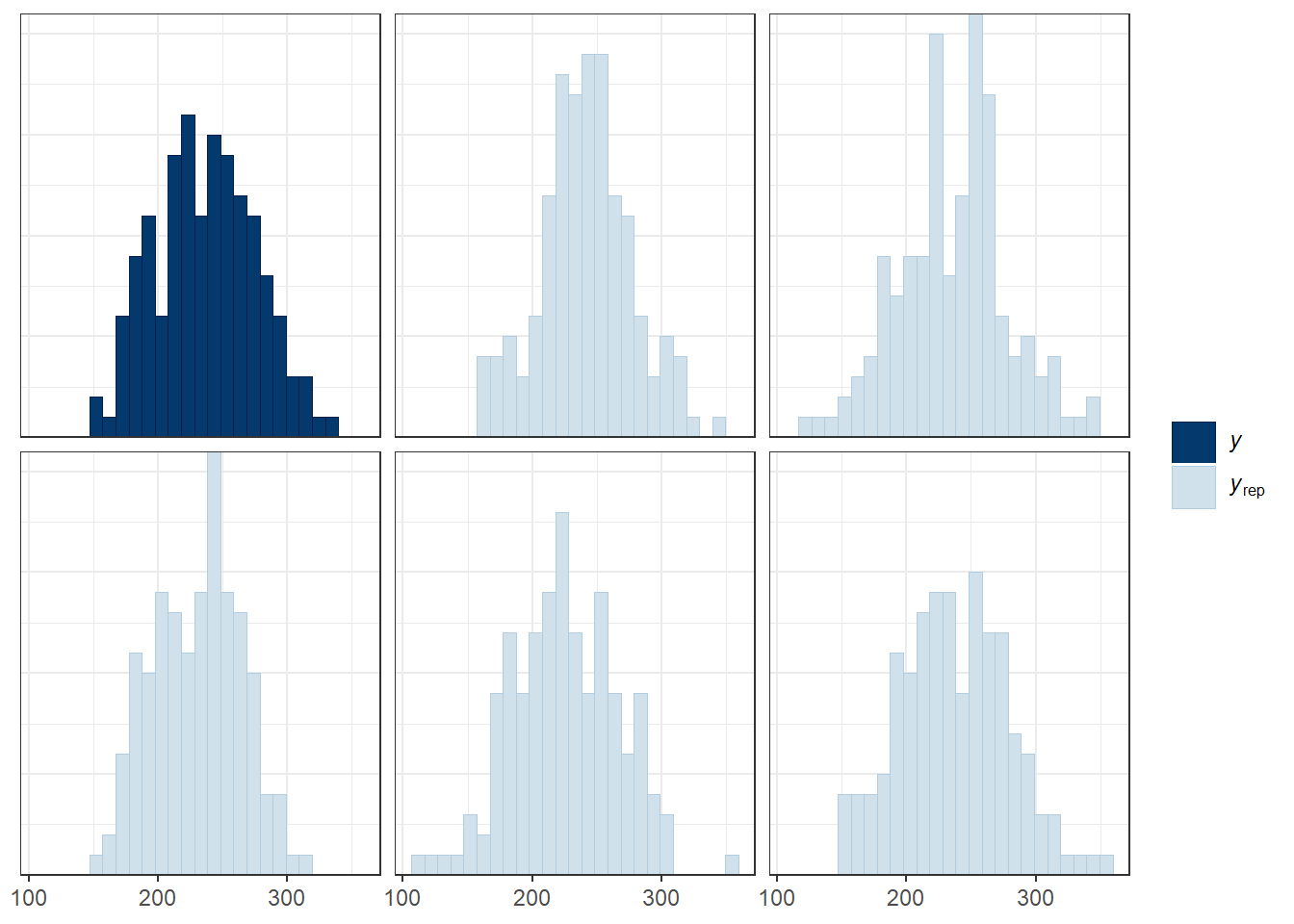

The idea is that if the model is a good fit to the data we should be able to generate data \(y_{rep}\) from the posterior predictive distribution that looks a lot like the observed data \(y\). That is, given \(y\), the \(y_{rep}\) we generate should look plausible. We’d worry a bit if this plot showed histograms that were wildly different from one another.

Another useful plot (shown below) made using pp_check shows the distribution of a test quantity \(T(y_{rep})\) compared to \(T(y)\), the value of the quantity in the observed data. I like this scatterplot version which allows us to look at where the simulations’ mean and standard deviation fall compared to what the observed totchol values show us.

pp_check(m2, plotfun = "stat_2d", stat = c("mean", "sd"))

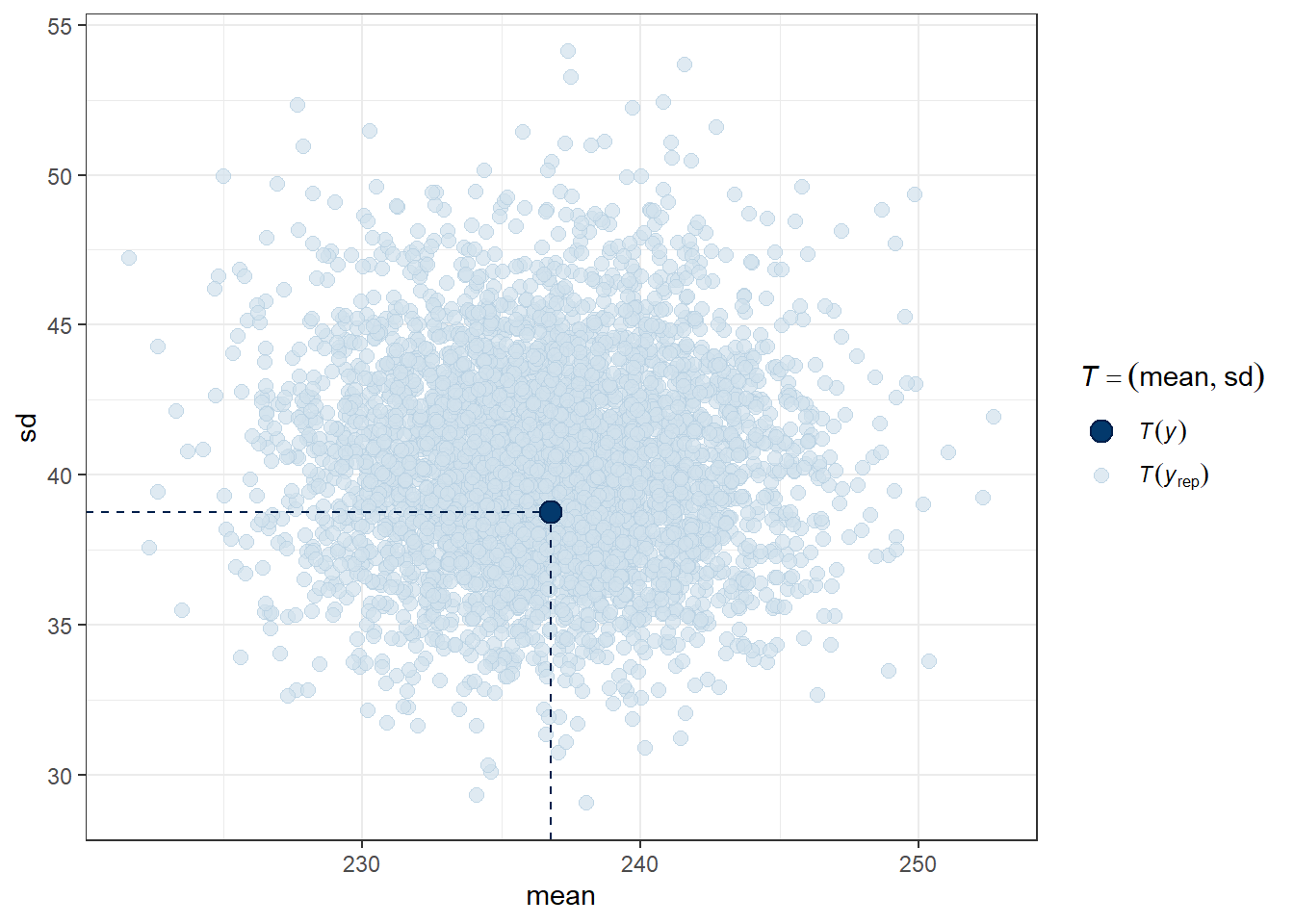
We can see that the cloud of simulated means and standard deviations has the observed statistics near its center, although perhaps the standard deviations are a bit higher than we might like to see, typically. Ideally, the dot would be right in the center of this cloud of simulated results.