15  A Model for Prostate Cancer

15.1 R Setup Used Here

knitr::opts_chunk$set(comment = NA)

library(broom)
library(rms)
library(tidyverse) 

theme_set(theme_bw())

15.1.1 Data Load

prost <- read_csv("data/prost.csv", show_col_types = FALSE) 

15.2 Data Load and Background

The data in prost.csv is derived from Stamey et al. (1989) who examined the relationship between the level of prostate-specific antigen and a number of clinical measures in 97 men who were about to receive a radical prostatectomy. The prost data, as I’ll name it in R, contains 97 rows and 11 columns.

prost

# A tibble: 97 × 10
   subject   lpsa lcavol lweight   age bph      svi   lcp gleason pgg45
     <dbl>  <dbl>  <dbl>   <dbl> <dbl> <chr>  <dbl> <dbl> <chr>   <dbl>
 1       1 -0.431 -0.580    2.77    50 Low        0 -1.39 6           0
 2       2 -0.163 -0.994    3.32    58 Low        0 -1.39 6           0
 3       3 -0.163 -0.511    2.69    74 Low        0 -1.39 7          20
 4       4 -0.163 -1.20     3.28    58 Low        0 -1.39 6           0
 5       5  0.372  0.751    3.43    62 Low        0 -1.39 6           0
 6       6  0.765 -1.05     3.23    50 Low        0 -1.39 6           0
 7       7  0.765  0.737    3.47    64 Medium     0 -1.39 6           0
 8       8  0.854  0.693    3.54    58 High       0 -1.39 6           0
 9       9  1.05  -0.777    3.54    47 Low        0 -1.39 6           0
10      10  1.05   0.223    3.24    63 Low        0 -1.39 6           0
# ℹ 87 more rows

Note that a related prost data frame is also available as part of several R packages, including the faraway package, but there is an error in the lweight data for subject 32 in those presentations. The value of lweight for subject 32 should not be 6.1, corresponding to a prostate that is 449 grams in size, but instead the lweight value should be 3.804438, corresponding to a 44.9 gram prostate¹.

I’ve also changed the gleason and bph variables from their presentation in other settings, to let me teach some additional details.

15.3 Code Book

Variable	Description
subject	subject number (1 to 97)
lpsa	log(prostate specific antigen in ng/ml), our outcome
lcavol	log(cancer volume in cm3)
lweight	log(prostate weight, in g)
age	age
bph	benign prostatic hyperplasia amount (Low, Medium, or High)
svi	seminal vesicle invasion (1 = yes, 0 = no)
lcp	log(capsular penetration, in cm)
gleason	combined Gleason score (6, 7, or > 7 here)
pgg45	percentage Gleason scores 4 or 5

Notes:

• in general, higher levels of PSA are stronger indicators of prostate cancer. An old standard (established almost exclusively with testing in white males, and definitely flawed) suggested that values below 4 were normal, and above 4 needed further testing. A PSA of 4 corresponds to an lpsa of 1.39.
• all logarithms are natural (base e) logarithms, obtained in R with the function log()
• all variables other than subject and lpsa are candidate predictors
• the gleason variable captures the highest combined Gleason score[^Scores range (in these data) from 6 (a well-differentiated, or low-grade cancer) to 9 (a high-grade cancer), although the maximum possible score is 10. 6 is the lowest score used for cancerous prostates. As this combination value increases, the rate at which the cancer grows and spreads should increase. This score refers to the combined Gleason grade, which is based on the sum of two areas (each scored 1-5) that make up most of the cancer.] in a biopsy, and higher scores indicate more aggressive cancer cells. It’s stored here as 6, 7, or > 7.
• the pgg45 variable captures the percentage of individual Gleason scores[^The 1-5 scale for individual biopsies are defined so that 1 indicates something that looks like normal prostate tissue, and 5 indicates that the cells and their growth patterns look very abnormal. In this study, the percentage of 4s and 5s shown in the data appears to be based on 5-20 individual scores in most subjects.] that are 4 or 5, on a 1-5 scale, where higher scores indicate more abnormal cells.

15.4 Additions for Later Use

The code below adds to the prost tibble:

• a factor version of the svi variable, called svi_f, with levels No and Yes,
• a factor version of gleason called gleason_f, with the levels ordered > 7, 7, and finally 6,
• a factor version of bph called bph_f, with levels ordered Low, Medium, High,
• a centered version of lcavol called lcavol_c,
• exponentiated cavol and psa results derived from the natural logarithms lcavol and lpsa.

prost <- prost |>
    mutate(svi_f = fct_recode(factor(svi), "No" = "0", "Yes" = "1"),
           gleason_f = fct_relevel(gleason, c("> 7", "7", "6")),
           bph_f = fct_relevel(bph, c("Low", "Medium", "High")),
           lcavol_c = lcavol - mean(lcavol),
           cavol = exp(lcavol),
           psa = exp(lpsa))

glimpse(prost)

Rows: 97
Columns: 16
$ subject   <dbl> 1, 2, 3, 4, 5, 6, 7, 8, 9, 10, 11, 12, 13, 14, 15, 16, 17, 1…
$ lpsa      <dbl> -0.4307829, -0.1625189, -0.1625189, -0.1625189, 0.3715636, 0…
$ lcavol    <dbl> -0.5798185, -0.9942523, -0.5108256, -1.2039728, 0.7514161, -…
$ lweight   <dbl> 2.769459, 3.319626, 2.691243, 3.282789, 3.432373, 3.228826, …
$ age       <dbl> 50, 58, 74, 58, 62, 50, 64, 58, 47, 63, 65, 63, 63, 67, 57, …
$ bph       <chr> "Low", "Low", "Low", "Low", "Low", "Low", "Medium", "High", …
$ svi       <dbl> 0, 0, 0, 0, 0, 0, 0, 0, 0, 0, 0, 0, 0, 0, 0, 0, 0, 0, 0, 0, …
$ lcp       <dbl> -1.3862944, -1.3862944, -1.3862944, -1.3862944, -1.3862944, …
$ gleason   <chr> "6", "6", "7", "6", "6", "6", "6", "6", "6", "6", "6", "6", …
$ pgg45     <dbl> 0, 0, 20, 0, 0, 0, 0, 0, 0, 0, 0, 0, 30, 5, 5, 0, 30, 0, 0, …
$ svi_f     <fct> No, No, No, No, No, No, No, No, No, No, No, No, No, No, No, …
$ gleason_f <fct> 6, 6, 7, 6, 6, 6, 6, 6, 6, 6, 6, 6, 7, 7, 7, 6, 7, 6, 6, 6, …
$ bph_f     <fct> Low, Low, Low, Low, Low, Low, Medium, High, Low, Low, Low, M…
$ lcavol_c  <dbl> -1.9298281, -2.3442619, -1.8608352, -2.5539824, -0.5985935, …
$ cavol     <dbl> 0.56, 0.37, 0.60, 0.30, 2.12, 0.35, 2.09, 2.00, 0.46, 1.25, …
$ psa       <dbl> 0.65, 0.85, 0.85, 0.85, 1.45, 2.15, 2.15, 2.35, 2.85, 2.85, …

15.5 Fitting and Evaluating a Two-Predictor Model

To begin, let’s use two predictors (lcavol and svi) and their interaction in a linear regression model that predicts lpsa. I’ll call this model prost_A

Earlier, we centered the lcavol values to facilitate interpretation of the terms. I’ll use that centered version (called lcavol_c) of the quantitative predictor, and the 1/0 version of the svi variable[^We could certainly use the factor version of svi here, but it won’t change the model in any meaningful way. There’s no distinction in model fitting via lm between a 0/1 numeric variable and a No/Yes factor variable. The factor version of this information will be useful elsewhere, for instance in plotting the model.].

prost_A <- lm(lpsa ~ lcavol_c * svi, data = prost)
summary(prost_A)

Call:
lm(formula = lpsa ~ lcavol_c * svi, data = prost)

Residuals:
    Min      1Q  Median      3Q     Max 
-1.6305 -0.5007  0.1266  0.4886  1.6847 

Coefficients:
             Estimate Std. Error t value Pr(>|t|)    
(Intercept)   2.33134    0.09128  25.540  < 2e-16 ***
lcavol_c      0.58640    0.08207   7.145 1.98e-10 ***
svi           0.60132    0.35833   1.678   0.0967 .  
lcavol_c:svi  0.06479    0.26614   0.243   0.8082    
---
Signif. codes:  0 '***' 0.001 '**' 0.01 '*' 0.05 '.' 0.1 ' ' 1

Residual standard error: 0.7595 on 93 degrees of freedom
Multiple R-squared:  0.5806,    Adjusted R-squared:  0.5671 
F-statistic: 42.92 on 3 and 93 DF,  p-value: < 2.2e-16

15.5.1 Using tidy

It can be very useful to build a data frame of the model’s results. We can use the tidy function in the broom package to do so.

tidy(prost_A)

# A tibble: 4 × 5
  term         estimate std.error statistic  p.value
  <chr>           <dbl>     <dbl>     <dbl>    <dbl>
1 (Intercept)    2.33      0.0913    25.5   8.25e-44
2 lcavol_c       0.586     0.0821     7.15  1.98e-10
3 svi            0.601     0.358      1.68  9.67e- 2
4 lcavol_c:svi   0.0648    0.266      0.243 8.08e- 1

This makes it much easier to pull out individual elements of the model fit.

For example, to specify the coefficient for svi, rounded to three decimal places, I could use

tidy(prost_A) |> filter(term == "svi") |> select(estimate) |> round(3)

• The result is 0.601.
• If you look at the Markdown file, you’ll see that the number shown in the bullet point above this one was generated using inline R code, and the function specified above.

15.5.2 Interpretation

1. The intercept, 2.33, for the model is the predicted value of lpsa when lcavol is at its average and there is no seminal vesicle invasion (e.g. svi = 0).
2. The coefficient for lcavol_c, 0.59, is the predicted change in lpsa associated with a one unit increase in lcavol (or lcavol_c) when there is no seminal vesicle invasion.
3. The coefficient for svi, 0.6, is the predicted change in lpsa associated with having no svi to having an svi while the lcavol remains at its average.
4. The coefficient for lcavol_c:svi, the product term, which is 0.06, is the difference in the slope of lcavol_c for a subject with svi as compared to one with no svi.

15.6 Exploring Model prost_A

The glance function from the broom package builds a nice one-row summary for the model.

glance(prost_A)

# A tibble: 1 × 12
  r.squared adj.r.squared sigma statistic  p.value    df logLik   AIC   BIC
      <dbl>         <dbl> <dbl>     <dbl>    <dbl> <dbl>  <dbl> <dbl> <dbl>
1     0.581         0.567 0.759      42.9 1.68e-17     3  -109.  228.  241.
# ℹ 3 more variables: deviance <dbl>, df.residual <int>, nobs <int>

This summary includes, in order,

• the model \(R^2\), adjusted \(R^2\) and \(\hat{\sigma}\), the residual standard deviation,
• the ANOVA F statistic and associated p value,
• the number of degrees of freedom used by the model, and its log-likelihood ratio
• the model’s AIC (Akaike Information Criterion) and BIC (Bayesian Information Criterion)
• the model’s deviance statistic and residual degrees of freedom

15.6.1 summary for Model prost_A

If necessary, we can also run summary on this prost_A object to pick up some additional summaries. Since the svi variable is binary, the interaction term is, too, so the t test here and the F test in the ANOVA yield the same result.

summary(prost_A)

Call:
lm(formula = lpsa ~ lcavol_c * svi, data = prost)

Residuals:
    Min      1Q  Median      3Q     Max 
-1.6305 -0.5007  0.1266  0.4886  1.6847 

Coefficients:
             Estimate Std. Error t value Pr(>|t|)    
(Intercept)   2.33134    0.09128  25.540  < 2e-16 ***
lcavol_c      0.58640    0.08207   7.145 1.98e-10 ***
svi           0.60132    0.35833   1.678   0.0967 .  
lcavol_c:svi  0.06479    0.26614   0.243   0.8082    
---
Signif. codes:  0 '***' 0.001 '**' 0.01 '*' 0.05 '.' 0.1 ' ' 1

Residual standard error: 0.7595 on 93 degrees of freedom
Multiple R-squared:  0.5806,    Adjusted R-squared:  0.5671 
F-statistic: 42.92 on 3 and 93 DF,  p-value: < 2.2e-16

If you’ve forgotten the details of the pieces of this summary, review the Part C Notes from 431.

15.6.2 Adjusted \(R^2\)

\(R^2\) is greedy.

• \(R^2\) will always suggest that we make our models as big as possible, often including variables of dubious predictive value.
• As a result, there are various methods for penalizing \(R^2\) so that we wind up with smaller models.
• The adjusted \(R^2\) is often a useful way to compare multiple models for the same response.
  • \(R^2_{adj} = 1 - \frac{(1-R^2)(n - 1)}{n - k}\), where \(n\) = the number of observations and \(k\) is the number of coefficients estimated by the regression (including the intercept and any slopes).
  • So, in this case, \(R^2_{adj} = 1 - \frac{(1 - 0.5806)(97 - 1)}{97 - 4} = 0.5671\)
  • The adjusted \(R^2\) value is not, technically, a proportion of anything, but it is comparable across models for the same outcome.
  • The adjusted \(R^2\) will always be less than the (unadjusted) \(R^2\).

15.6.3 Coefficient Confidence Intervals

Here are the 90% confidence intervals for the coefficients in Model A. Adjust the level to get different intervals.

confint(prost_A, level = 0.90)

                     5 %      95 %
(Intercept)   2.17968697 2.4830012
lcavol_c      0.45004577 0.7227462
svi           0.00599401 1.1966454
lcavol_c:svi -0.37737623 0.5069622

What can we conclude from this about the utility of the interaction term?

15.6.4 ANOVA for Model prost_A

The interaction term appears unnecessary. We might wind up fitting the model without it. A complete ANOVA test is available, including a p value, if you want it.

anova(prost_A)

Analysis of Variance Table

Response: lpsa
             Df Sum Sq Mean Sq  F value    Pr(>F)    
lcavol_c      1 69.003  69.003 119.6289 < 2.2e-16 ***
svi           1  5.237   5.237   9.0801  0.003329 ** 
lcavol_c:svi  1  0.034   0.034   0.0593  0.808191    
Residuals    93 53.643   0.577                       
---
Signif. codes:  0 '***' 0.001 '**' 0.01 '*' 0.05 '.' 0.1 ' ' 1

Note that the anova approach for a lm object is sequential. The first row shows the impact of lcavol_c as compared to a model with no predictors (just an intercept). The second row shows the impact of adding svi to a model that already contains lcavol_c. The third row shows the impact of adding the interaction (product) term to the model with the two main effects. So the order in which the variables are added to the regression model matters for this ANOVA. The F tests here describe the incremental impact of each covariate in turn.

15.6.5 Residuals, Fitted Values and Standard Errors with augment

The augment function in the broom package builds a data frame including the data used in the model, along with predictions (fitted values), residuals and other useful information.

prost_A_aug <- augment(prost_A)
summary(prost_A_aug)

      lpsa            lcavol_c             svi            .fitted      
 Min.   :-0.4308   Min.   :-2.69708   Min.   :0.0000   Min.   :0.7498  
 1st Qu.: 1.7317   1st Qu.:-0.83719   1st Qu.:0.0000   1st Qu.:1.8404  
 Median : 2.5915   Median : 0.09691   Median :0.0000   Median :2.3950  
 Mean   : 2.4784   Mean   : 0.00000   Mean   :0.2165   Mean   :2.4784  
 3rd Qu.: 3.0564   3rd Qu.: 0.77703   3rd Qu.:0.0000   3rd Qu.:3.0709  
 Max.   : 5.5829   Max.   : 2.47099   Max.   :1.0000   Max.   :4.5417  
     .resid             .hat             .sigma          .cooksd         
 Min.   :-1.6305   Min.   :0.01316   Min.   :0.7423   Min.   :0.0000069  
 1st Qu.:-0.5007   1st Qu.:0.01562   1st Qu.:0.7569   1st Qu.:0.0007837  
 Median : 0.1266   Median :0.02498   Median :0.7617   Median :0.0034699  
 Mean   : 0.0000   Mean   :0.04124   Mean   :0.7595   Mean   :0.0111314  
 3rd Qu.: 0.4886   3rd Qu.:0.04939   3rd Qu.:0.7631   3rd Qu.:0.0103533  
 Max.   : 1.6847   Max.   :0.24627   Max.   :0.7636   Max.   :0.1341093  
   .std.resid       
 Min.   :-2.194508  
 1st Qu.:-0.687945  
 Median : 0.168917  
 Mean   : 0.001249  
 3rd Qu.: 0.653612  
 Max.   : 2.261830  

Elements shown here include:

• .fitted Fitted values of model (or predicted values)
• .se.fit Standard errors of fitted values
• .resid Residuals (observed - fitted values)
• .hat Diagonal of the hat matrix (these indicate leverage - points with high leverage indicate unusual combinations of predictors - values more than 2-3 times the mean leverage are worth some study - leverage is always between 0 and 1, and measures the amount by which the predicted value would change if the observation’s y value was increased by one unit - a point with leverage 1 would cause the line to follow that point perfectly)
• .sigma Estimate of residual standard deviation when corresponding observation is dropped from model
• .cooksd Cook’s distance, which helps identify influential points (values of Cook’s d > 0.5 may be influential, values > 1.0 almost certainly are - an influential point changes the fit substantially when it is removed from the data)
• .std.resid Standardized residuals (values above 2 in absolute value are worth some study - treat these as normal deviates [Z scores], essentially)

See ?augment.lm in R for more details.

15.6.6 Making Predictions with prost_A

Suppose we want to predict the lpsa for a patient with cancer volume equal to this group’s mean, for both a patient with and without seminal vesicle invasion, and in each case, we want to use a 90% prediction interval?

newdata <- data.frame(lcavol_c = c(0,0), svi = c(0,1))
predict(prost_A, newdata, interval = "prediction", level = 0.90)

       fit      lwr      upr
1 2.331344 1.060462 3.602226
2 2.932664 1.545742 4.319586

Since the predicted value in fit refers to the natural logarithm of PSA, to make the predictions in terms of PSA, we would need to exponentiate. The code below will accomplish that task.

pred <- predict(prost_A, newdata, interval = "prediction", level = 0.90)
exp(pred)

       fit      lwr      upr
1 10.29177 2.887706 36.67978
2 18.77758 4.691450 75.15750

15.7 Plotting Model prost_A

15.7.0.1 Plot logs conventionally

Here, we’ll use ggplot2 to plot the logarithms of the variables as they came to us, on a conventional coordinate scale. Note that the lines are nearly parallel. What does this suggest about our Model A?

ggplot(prost, aes(x = lcavol, y = lpsa, group = svi_f, color = svi_f)) +
    geom_point() +
    geom_smooth(method = "lm", formula = y ~ x, se = FALSE) + 
    scale_color_discrete(name = "Seminal Vesicle Invasion?") +
    theme_bw() +
    labs(x = "Log (cancer volume, cc)", 
         y = "Log (Prostate Specific Antigen, ng/ml)", 
         title = "Two Predictor Model prost_A, including Interaction")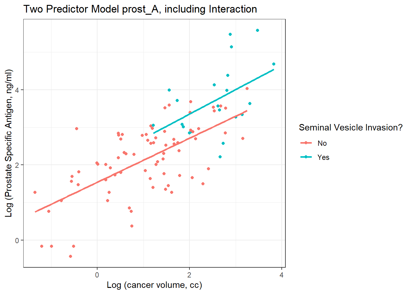

15.7.0.2 Plot on log-log scale

Another approach (which might be easier in some settings) would be to plot the raw values of Cancer Volume and PSA, but use logarithmic axes, again using the natural (base e) logarithm, as follows. If we use the default choice with `trans = “log”, we’ll find a need to select some useful break points for the grid, as I’ve done in what follows.

ggplot(prost, aes(x = cavol, y = psa, group = svi_f, color = svi_f)) +
    geom_point() +
    geom_smooth(method = "lm", formula = y ~ x, se = FALSE) + 
    scale_color_discrete(name = "Seminal Vesicle Invasion?") +
    scale_x_continuous(trans = "log", 
                       breaks = c(0.5, 1, 2, 5, 10, 25, 50)) +
    scale_y_continuous(trans = "log", 
                       breaks = c(1, 2, 4, 10, 25, 50, 100, 200)) +
    theme_bw() +
    labs(x = "Cancer volume, in cubic centimeters", 
         y = "Prostate Specific Antigen, in ng/ml", 
         title = "Two Predictor Model prost_A, including Interaction")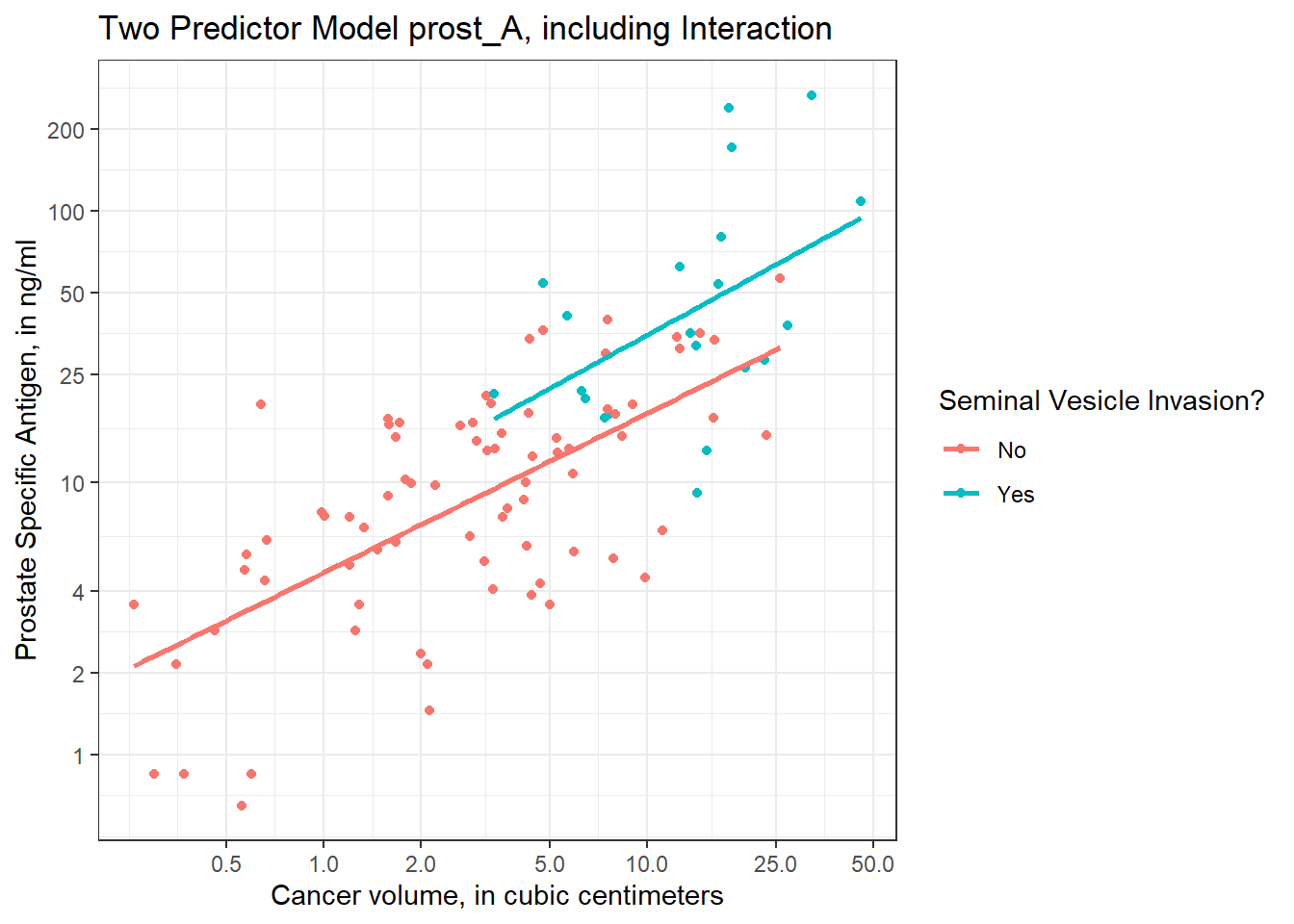

I’ve used the break point of 4 on the Y axis because of the old rule suggesting further testing for asymptomatic men with PSA of 4 or higher, but the other break points are arbitrary - they seemed to work for me, and used round numbers.

15.7.1 Residual Plots of prost_A

plot(prost_A, which = 1)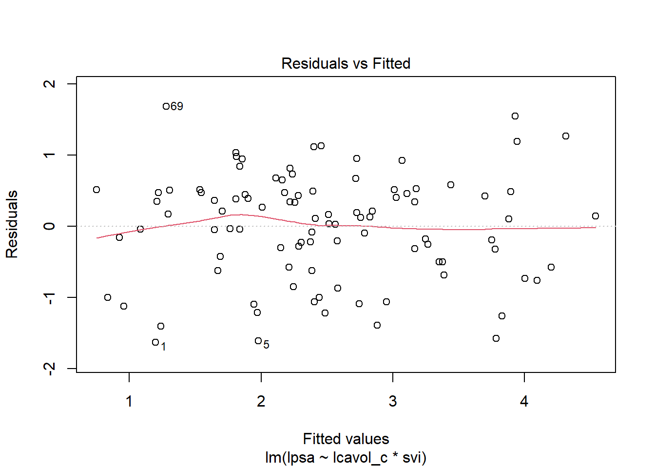

plot(prost_A, which = 5)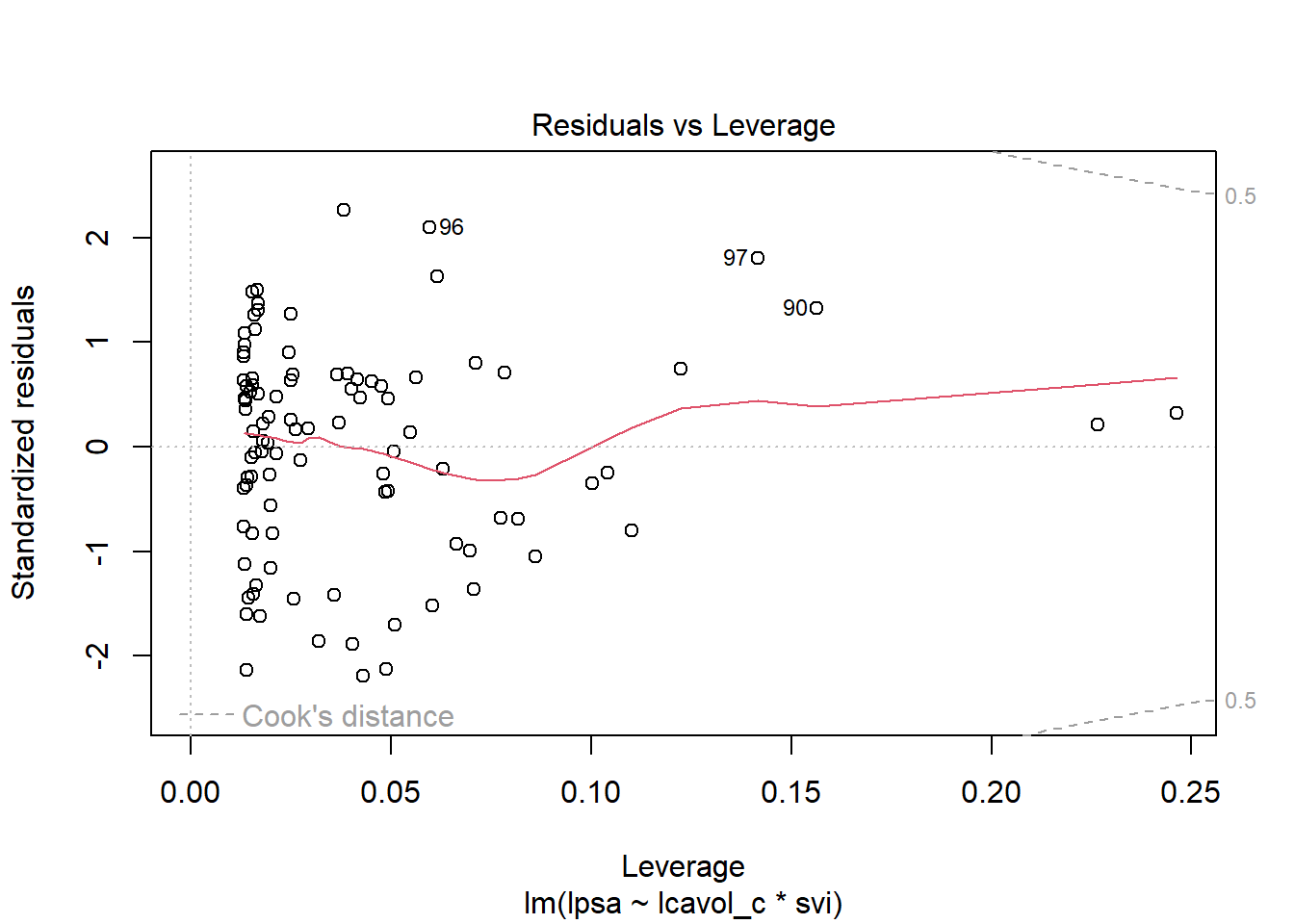

In our next Chapter, we’ll see how well this model can be validated.

Stamey, J. N. Kabalin, T. A. et al. 1989. “Prostate Specific Antigen in the Diagnosis and Treatment of Adenocarcinoma of the Prostate: II. Radical Prostatectomy Treated Patients.” Journal of Urology 141(5): 1076–83. https://www.ncbi.nlm.nih.gov/pubmed/2468795.

---

1. https://statweb.stanford.edu/~tibs/ElemStatLearn/ attributes the correction to Professor Stephen W. Link.