32  NEW!! A Few LASSO Ideas

32.1 R Setup Used Here

knitr::opts_chunk$set(comment = NA)

library(janitor)
library(broom)
library(car)
library(gt)
library(Hmisc)
library(MASS)
library(mosaic)
library(glmnet)
library(conflicted)
library(patchwork)
library(tidyverse) 

conflicts_prefer(dplyr::select)

theme_set(theme_bw())

32.1.1 Data Load

pollution <- read_csv("data/pollution.csv", show_col_types = FALSE) 

32.2 The pollution data

Consider again the pollution data set we developed in Chapter 13 which contains 15 independent variables and a measure of mortality, describing 60 US metropolitan areas in 1959-1961.

pollution

# A tibble: 60 × 16
      x1    x2    x3    x4    x5    x6    x7    x8    x9   x10   x11   x12   x13
   <dbl> <dbl> <dbl> <dbl> <dbl> <dbl> <dbl> <dbl> <dbl> <dbl> <dbl> <dbl> <dbl>
 1    13    49    68   7    3.36  12.2  90.7  2702   3    51.9   9.7   105    32
 2    28    32    81   7    3.27  12.1  81    3665   7.5  51.6  13.2     4     2
 3    10    55    70   7.3  3.11  12.1  88.9  3033   5.9  51    14     144    66
 4    43    32    74  10.1  3.38   9.5  79.2  3214   2.9  43.7  12      11     7
 5    25    12    73   9.2  3.28  12.1  83.1  2095   2    51.9   9.8    20    11
 6    35    46    85   7.1  3.22  11.8  79.9  1441  14.8  51.2  16.1     1     1
 7    60    67    82  10    2.98  11.5  88.6  4657  13.5  47.3  22.4     3     1
 8    11    53    68   9.2  2.99  12.1  90.6  4700   7.8  48.9  12.3   648   319
 9    31    24    72   9    3.37  10.9  82.8  3226   5.1  45.2  12.3     5     3
10    15    30    73   8.2  3.15  12.2  84.2  4824   4.7  53.1  12.7    17     8
# ℹ 50 more rows
# ℹ 3 more variables: x14 <dbl>, x15 <dbl>, y <dbl>

Here’s a codebook:

Variable	Description
y	Total Age Adjusted Mortality Rate
x1	Mean annual precipitation in inches
x2	Mean January temperature in degrees Fahrenheit
x3	Mean July temperature in degrees Fahrenheit
x4	Percent of 1960 SMSA population that is 65 years of age or over
x5	Population per household, 1960 SMSA
x6	Median school years completed for those over 25 in 1960 SMSA
x7	Percent of housing units that are found with facilities
x8	Population per square mile in urbanized area in 1960
x9	Percent of 1960 urbanized area population that is non-white
x10	Percent employment in white-collar occupations in 1960 urbanized area
x11	Percent of families with income under $30,000 in 1960 urbanized area
x12	Relative population potential of hydrocarbons, HC
x13	Relative pollution potential of oxides of nitrogen, NOx
x14	Relative pollution potential of sulfur dioxide, SO2
x15	Percent relative humidity, annual average at 1 p.m.

32.3 Should We Rescale any Predictors?

Let’s get some basic summary statistics for our candidate predictors. When we do, we see that variable x8 is roughy 100 times larger than all of our other predictors.

df_stats(~ x1 + x2 + x3 + x4 + x5 + x6 + x7 + x8 + x9 + 
           x10 + x11 + x12 + x13 + x14 + x15, data = pollution)

   response     min       Q1   median       Q3     max        mean           sd
1        x1   10.00   32.750   38.000   43.250   60.00   37.366667    9.9846775
2        x2   12.00   27.000   31.500   40.000   67.00   33.983333   10.1688985
3        x3   63.00   72.000   74.000   77.250   85.00   74.583333    4.7631768
4        x4    5.60    7.675    9.000    9.700   11.80    8.798333    1.4645520
5        x5    2.92    3.210    3.265    3.360    3.53    3.263167    0.1352523
6        x6    9.00   10.400   11.050   11.500   12.30   10.973333    0.8452994
7        x7   66.80   78.375   81.150   83.600   90.70   80.913333    5.1413731
8        x8 1441.00 3104.250 3567.000 4519.750 9699.00 3876.050000 1454.1023607
9        x9    0.80    4.950   10.400   15.650   38.50   11.870000    8.9211480
10      x10   33.80   43.250   45.500   49.525   59.70   46.081667    4.6130431
11      x11    9.40   12.000   13.200   15.150   26.40   14.373333    4.1600956
12      x12    1.00    7.000   14.500   30.250  648.00   37.850000   91.9776732
13      x13    1.00    4.000    9.000   23.750  319.00   22.650000   46.3332896
14      x14    1.00   11.000   30.000   69.000  278.00   53.766667   63.3904678
15      x15   38.00   55.000   57.000   60.000   73.00   57.666667    5.3699309
    n missing
1  60       0
2  60       0
3  60       0
4  60       0
5  60       0
6  60       0
7  60       0
8  60       0
9  60       0
10 60       0
11 60       0
12 60       0
13 60       0
14 60       0
15 60       0

Let’s dampen the size of that x8 variable down a little to make our coefficient comparisons easier later, by dividing all of the x8 values by 100.

pollution <- pollution |>
  mutate(x8 = x8/100)

32.4 A Kitchen Sink Model

We’ll begin by fitting the obviously underpowered model with all 15 main effects used to predict our outcome.

mod_sink <- lm(y ~ x1 + x2 + x3 + x4 + x5 + x6 + x7 + x8 + x9 + 
                 x10 + x11 + x12 + x13 + x14 + x15, 
               data = pollution)

32.4.1 Considering an Outcome Transformation

boxcox(mod_sink)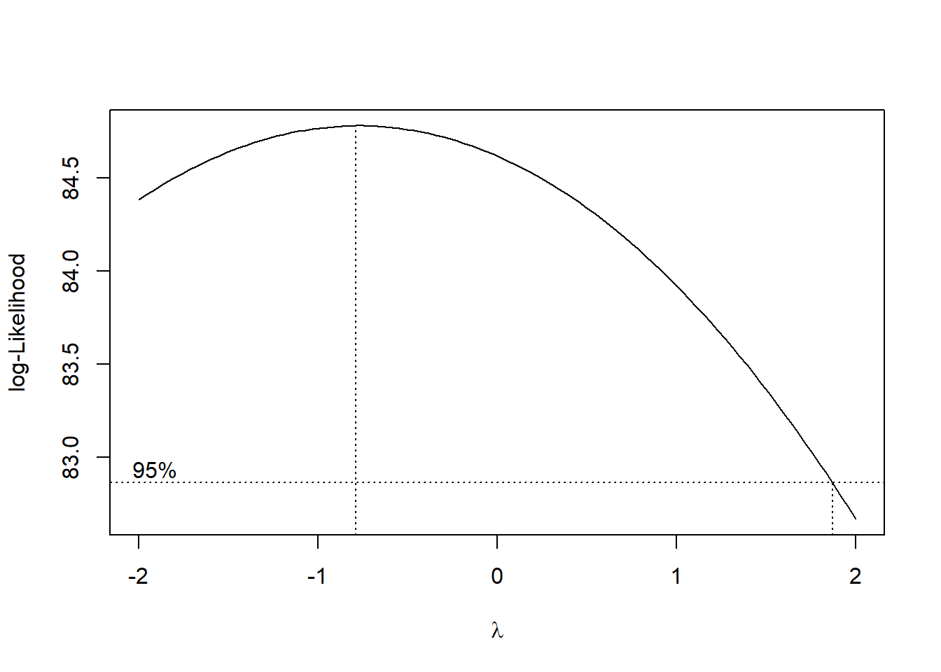

OK. In light of this Box-Cox plot, let’s consider taking the inverse of our outcome here. I’ll take that inverse and then standardize the result using the scale() function to both subtract the mean of the transformed outcome and divide by its standard deviation, so that our new outcome, which I’ll call out_std has mean 0, standard deviation 1, and a shape similar to that of the inverse of our \(y\).

pollution <- pollution |> 
  mutate(y_inverse = 1/y,
         out_std = scale(1/y, center = TRUE, scale = TRUE))

p1 <- ggplot(pollution, aes(x = y_inverse)) + geom_density()
p2 <- ggplot(pollution, aes(x = out_std)) + geom_density()

p1 / p2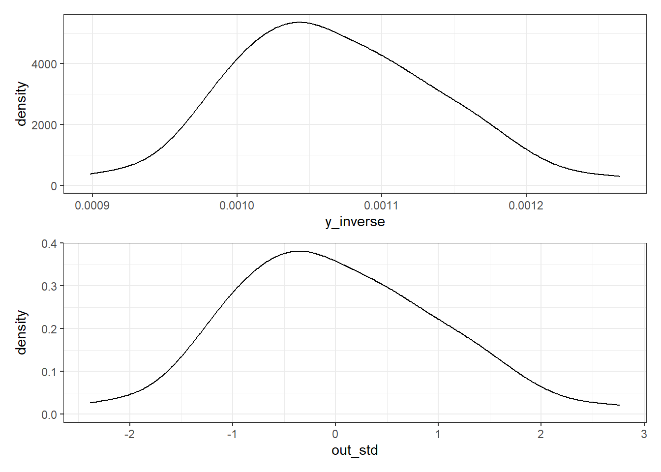

OK. So now, I’ll build a revised kitchen sink model to use this new outcome.

mod_sink2 <- lm(out_std ~ x1 + x2 + x3 + x4 + x5 + x6 + x7 + x8 + x9 + 
                 x10 + x11 + x12 + x13 + x14 + x15, data = pollution)

tidy(mod_sink2, conf.int = TRUE, conf.level = 0.9) |> 
  select(term, estimate, std.error, conf.low, conf.high, p.value) |>
  gt() |> fmt_number(decimals = 3)

term	estimate	std.error	conf.low	conf.high	p.value
(Intercept)	−15.899	6.886	−27.469	−4.328	0.026
x1	−0.035	0.015	−0.059	−0.011	0.020
x2	0.036	0.017	0.007	0.066	0.044
x3	0.055	0.030	0.005	0.105	0.074
x4	0.176	0.134	−0.049	0.400	0.196
x5	2.184	1.099	0.338	4.031	0.053
x6	0.225	0.187	−0.089	0.539	0.234
x7	0.016	0.028	−0.031	0.063	0.573
x8	−0.006	0.006	−0.017	0.005	0.351
x9	−0.070	0.021	−0.105	−0.035	0.002
x10	0.012	0.026	−0.031	0.056	0.636
x11	0.002	0.051	−0.084	0.087	0.974
x12	0.011	0.008	−0.002	0.024	0.160
x13	−0.022	0.016	−0.049	0.004	0.169
x14	−0.001	0.002	−0.005	0.003	0.549
x15	0.001	0.018	−0.029	0.032	0.936

Does this new model show a strong fit to the data?

glance(mod_sink2) |> select(r.squared:p.value, df, df.residual, nobs) |>
  gt() |> fmt_number(r.squared:p.value, decimals = 3)

r.squared	adj.r.squared	sigma	statistic	p.value	df	df.residual	nobs
0.774	0.698	0.550	10.070	0.000	15	44	60

glance(mod_sink2) |> select(logLik, AIC, BIC, deviance) |> gt() |> 
  fmt_number(decimals = 2)

logLik	AIC	BIC	deviance
−39.96	113.92	149.52	13.31

32.4.2 How much collinearity are we dealing with?

vif(mod_sink2)

        x1         x2         x3         x4         x5         x6         x7 
  4.113888   6.143551   3.967774   7.470045   4.307618   4.860538   3.994781 
        x8         x9        x10        x11        x12        x13        x14 
  1.658281   6.779599   2.841582   8.717068  98.639935 104.982405   4.228929 
       x15 
  1.907092 

Clearly, we have some enormous collinearity to deal with, given that we have many VIFs over 5, some even over 100.

So a reduction in the size of the model seems appealing for multiple reasons.

32.5 Using the LASSO to suggest a smaller model

To begin, we will create a data matrix for our predictors, as follows:

pred_x <- model.matrix(mod_sink2)

Next, we create a matrix of our outcome.

out_y <- pollution |> select(out_std) |> as.matrix()

The LASSO involves both a cross-validation step, and a fitting step. Here’s the code we’ll use in this case:

set.seed(123456)

cv_poll1 <- cv.glmnet(pred_x, out_y, type.measure = "mse", nfolds = 10)

mod_las1 <- glmnet(pred_x, out_y, alpha = 1, lambda = cv_poll1$lambda.min)

Now, let’s look at what the LASSO does. As we can see from the tidied output below, some predictors are dropped from the model, while others have their coefficients shrunk towards zero as compared to what we saw in the “kitchen sink” model.

tidy(mod_las1) |> gt()

term	step	estimate	lambda	dev.ratio
(Intercept)	1	-2.345226117	0.03783146	0.7335261
x1	1	-0.026289494	0.03783146	0.7335261
x2	1	0.020872173	0.03783146	0.7335261
x3	1	0.017666053	0.03783146	0.7335261
x6	1	0.101973313	0.03783146	0.7335261
x7	1	0.012515424	0.03783146	0.7335261
x8	1	-0.006425945	0.03783146	0.7335261
x9	1	-0.060226425	0.03783146	0.7335261
x10	1	0.007342706	0.03783146	0.7335261
x14	1	-0.003819796	0.03783146	0.7335261

This new LASSO model includes only 9 of the original 15 predictors.

32.6 Would the 9-predictor model be a big improvement?

Suppose we fit a new model inspired by this LASSO. It’s still just a linear model, with no shrinkage, here.

mod_3 <- lm(out_std ~ x1 + x2 + x3 + x6 + x7 + x8 + x9 + x10 + x14, 
            data = pollution)

vif(mod_3)

      x1       x2       x3       x6       x7       x8       x9      x10 
1.850485 1.548039 1.867603 3.899194 2.318288 1.479122 2.281879 2.333836 
     x14 
1.609159 

Well, the collinearity is certainly much improved.

tidy(mod_3, conf.int = TRUE, conf.level = 0.9) |> 
  select(term, estimate, std.error, conf.low, conf.high, p.value) |>
  gt() |> fmt_number(decimals = 3)

term	estimate	std.error	conf.low	conf.high	p.value
(Intercept)	−4.122	2.254	−7.900	−0.344	0.073
x1	−0.031	0.010	−0.048	−0.015	0.002
x2	0.024	0.009	0.010	0.039	0.007
x3	0.040	0.020	0.005	0.074	0.058
x6	0.057	0.166	−0.222	0.335	0.734
x7	0.021	0.021	−0.014	0.056	0.328
x8	−0.009	0.006	−0.019	0.001	0.129
x9	−0.069	0.012	−0.090	−0.049	0.000
x10	0.013	0.024	−0.026	0.053	0.581
x14	−0.004	0.001	−0.006	−0.002	0.007

Does this new model show a strong fit to the data?

glance(mod_3) |> select(r.squared:p.value, df, df.residual, nobs) |>
  gt() |> fmt_number(r.squared:p.value, decimals = 3)

r.squared	adj.r.squared	sigma	statistic	p.value	df	df.residual	nobs
0.747	0.702	0.546	16.413	0.000	9	50	60

glance(mod_3) |> select(logLik, AIC, BIC, deviance) |> gt() |> 
  fmt_number(decimals = 2)

logLik	AIC	BIC	deviance
−43.39	108.78	131.81	14.92

Finally, here’s a set of plots for regression diagnostics. How do things look?

par(mfrow = c(2,2))
plot(mod_3)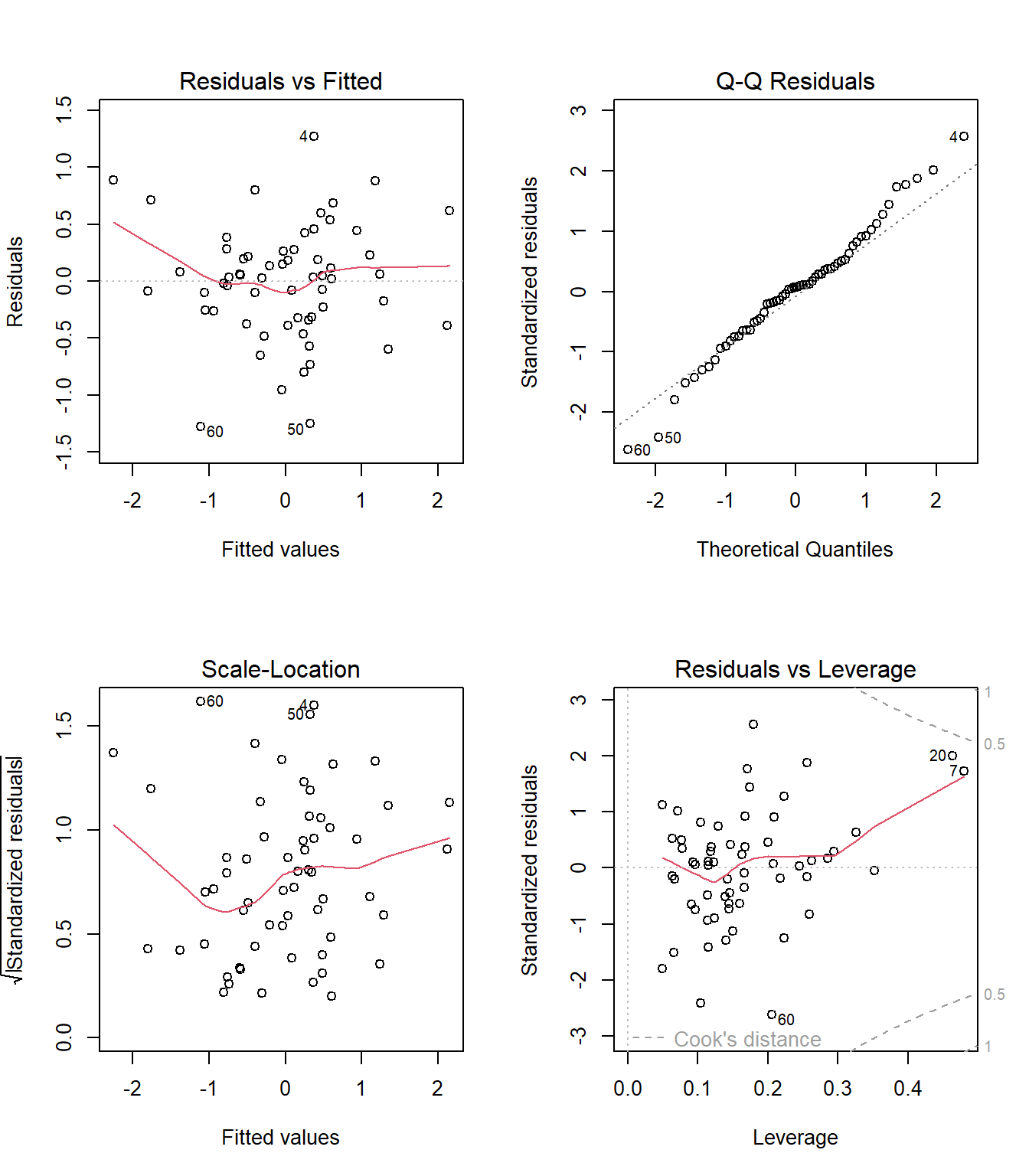

32.7 Using Stepwise Regression to suggest a smaller model

mod_4 <- step(mod_sink2)

Start:  AIC=-58.35
out_std ~ x1 + x2 + x3 + x4 + x5 + x6 + x7 + x8 + x9 + x10 + 
    x11 + x12 + x13 + x14 + x15

       Df Sum of Sq    RSS     AIC
- x11   1    0.0003 13.310 -60.351
- x15   1    0.0020 13.311 -60.344
- x10   1    0.0689 13.378 -60.043
- x7    1    0.0976 13.407 -59.914
- x14   1    0.1102 13.420 -59.858
- x8    1    0.2693 13.579 -59.151
- x6    1    0.4401 13.749 -58.401
<none>              13.309 -58.353
- x4    1    0.5226 13.832 -58.042
- x13   1    0.5906 13.900 -57.747
- x12   1    0.6186 13.928 -57.627
- x3    1    1.0145 14.324 -55.945
- x5    1    1.1956 14.505 -55.191
- x2    1    1.3063 14.616 -54.735
- x1    1    1.7574 15.067 -52.911
- x9    1    3.4141 16.723 -46.652

Step:  AIC=-60.35
out_std ~ x1 + x2 + x3 + x4 + x5 + x6 + x7 + x8 + x9 + x10 + 
    x12 + x13 + x14 + x15

       Df Sum of Sq    RSS     AIC
- x15   1    0.0017 13.311 -62.343
- x10   1    0.0696 13.379 -62.038
- x14   1    0.1119 13.422 -61.849
- x7    1    0.1411 13.451 -61.719
- x8    1    0.2752 13.585 -61.123
- x6    1    0.4398 13.749 -60.401
<none>              13.310 -60.351
- x13   1    0.5905 13.900 -59.747
- x4    1    0.6048 13.915 -59.685
- x12   1    0.6202 13.930 -59.618
- x3    1    1.0419 14.352 -57.829
- x5    1    1.2132 14.523 -57.117
- x1    1    1.8672 15.177 -54.474
- x2    1    2.3995 15.709 -52.406
- x9    1    4.5934 17.903 -44.562

Step:  AIC=-62.34
out_std ~ x1 + x2 + x3 + x4 + x5 + x6 + x7 + x8 + x9 + x10 + 
    x12 + x13 + x14

       Df Sum of Sq    RSS     AIC
- x10   1    0.0680 13.380 -64.037
- x14   1    0.1102 13.422 -63.849
- x7    1    0.1398 13.451 -63.717
- x8    1    0.2800 13.591 -63.094
<none>              13.311 -62.343
- x6    1    0.4538 13.765 -62.332
- x4    1    0.6066 13.918 -61.669
- x13   1    0.6080 13.919 -61.664
- x12   1    0.6251 13.937 -61.590
- x5    1    1.2142 14.526 -59.106
- x3    1    1.5567 14.868 -57.707
- x1    1    1.8661 15.178 -56.472
- x2    1    2.7077 16.019 -53.234
- x9    1    4.6990 18.010 -46.204

Step:  AIC=-64.04
out_std ~ x1 + x2 + x3 + x4 + x5 + x6 + x7 + x8 + x9 + x12 + 
    x13 + x14

       Df Sum of Sq    RSS     AIC
- x14   1    0.0750 13.454 -65.702
- x7    1    0.1158 13.495 -65.520
- x8    1    0.2459 13.625 -64.945
<none>              13.380 -64.037
- x4    1    0.6708 14.050 -63.102
- x12   1    0.7497 14.129 -62.766
- x13   1    0.7575 14.137 -62.733
- x6    1    1.1206 14.500 -61.212
- x5    1    1.1650 14.544 -61.028
- x3    1    1.6471 15.027 -59.071
- x1    1    1.9708 15.350 -57.793
- x2    1    2.8845 16.264 -54.323
- x9    1    4.6459 18.025 -48.154

Step:  AIC=-65.7
out_std ~ x1 + x2 + x3 + x4 + x5 + x6 + x7 + x8 + x9 + x12 + 
    x13

       Df Sum of Sq    RSS     AIC
- x7    1    0.0736 13.528 -67.375
- x8    1    0.2931 13.748 -66.409
<none>              13.454 -65.702
- x4    1    0.7633 14.218 -64.391
- x5    1    1.3276 14.782 -62.056
- x6    1    1.5095 14.964 -61.322
- x3    1    1.6936 15.148 -60.588
- x1    1    1.9047 15.359 -59.758
- x12   1    2.2433 15.698 -58.450
- x13   1    2.5554 16.010 -57.269
- x2    1    3.2927 16.747 -54.567
- x9    1    4.9296 18.384 -48.972

Step:  AIC=-67.37
out_std ~ x1 + x2 + x3 + x4 + x5 + x6 + x8 + x9 + x12 + x13

       Df Sum of Sq    RSS     AIC
- x8    1    0.2268 13.755 -68.377
<none>              13.528 -67.375
- x4    1    0.6973 14.225 -66.359
- x5    1    1.2978 14.826 -63.878
- x3    1    1.6230 15.151 -62.576
- x1    1    1.8418 15.370 -61.716
- x6    1    2.1350 15.663 -60.582
- x12   1    2.2355 15.764 -60.199
- x13   1    2.5168 16.045 -59.137
- x2    1    3.3522 16.880 -56.092
- x9    1    6.1854 19.713 -46.783

Step:  AIC=-68.38
out_std ~ x1 + x2 + x3 + x4 + x5 + x6 + x9 + x12 + x13

       Df Sum of Sq    RSS     AIC
<none>              13.755 -68.377
- x4    1    0.8670 14.622 -66.710
- x3    1    1.6985 15.453 -63.391
- x1    1    1.8777 15.633 -62.700
- x5    1    1.9839 15.739 -62.293
- x12   1    2.4622 16.217 -60.497
- x13   1    2.8317 16.587 -59.145
- x6    1    3.0868 16.842 -58.229
- x2    1    4.0486 17.803 -54.897
- x9    1    6.3106 20.065 -47.721

Here’s a summary of the fitted model after stepwise regression, which suggests a different set of 9 predictors.

tidy(mod_4, conf.int = TRUE, conf.level = 0.9) |> 
  select(term, estimate, std.error, conf.low, conf.high, p.value) |>
  gt() |> fmt_number(decimals = 3)

term	estimate	std.error	conf.low	conf.high	p.value
(Intercept)	−17.332	5.257	−26.142	−8.522	0.002
x1	−0.034	0.013	−0.057	−0.012	0.012
x2	0.042	0.011	0.024	0.060	0.000
x3	0.055	0.022	0.018	0.092	0.016
x4	0.200	0.113	0.011	0.388	0.082
x5	2.530	0.942	0.951	4.109	0.010
x6	0.373	0.111	0.186	0.559	0.002
x9	−0.073	0.015	−0.099	−0.048	0.000
x12	0.015	0.005	0.007	0.023	0.004
x13	−0.031	0.010	−0.047	−0.015	0.002

glance(mod_4) |> select(r.squared:p.value, df, df.residual, nobs) |>
  gt() |> fmt_number(r.squared:p.value, decimals = 3)

r.squared	adj.r.squared	sigma	statistic	p.value	df	df.residual	nobs
0.767	0.725	0.524	18.274	0.000	9	50	60

glance(mod_4) |> select(logLik, AIC, BIC, deviance) |> gt() |> 
  fmt_number(decimals = 2)

logLik	AIC	BIC	deviance
−40.95	103.90	126.93	13.75

How is the collinearity in this model?

vif(mod_4)

       x1        x2        x3        x4        x5        x6        x9       x12 
 3.724589  2.666789  2.359891  5.826631  3.483085  1.898922  3.981753 45.943057 
      x13 
42.500579 

That looks more troubling to me, at least as compared to mod_3. How about the residual plots? Do those for mod_4 below look meaningfully different from the ones we built for our LASSO-inspired model mod_3?

par(mfrow = c(2,2))
plot(mod_4)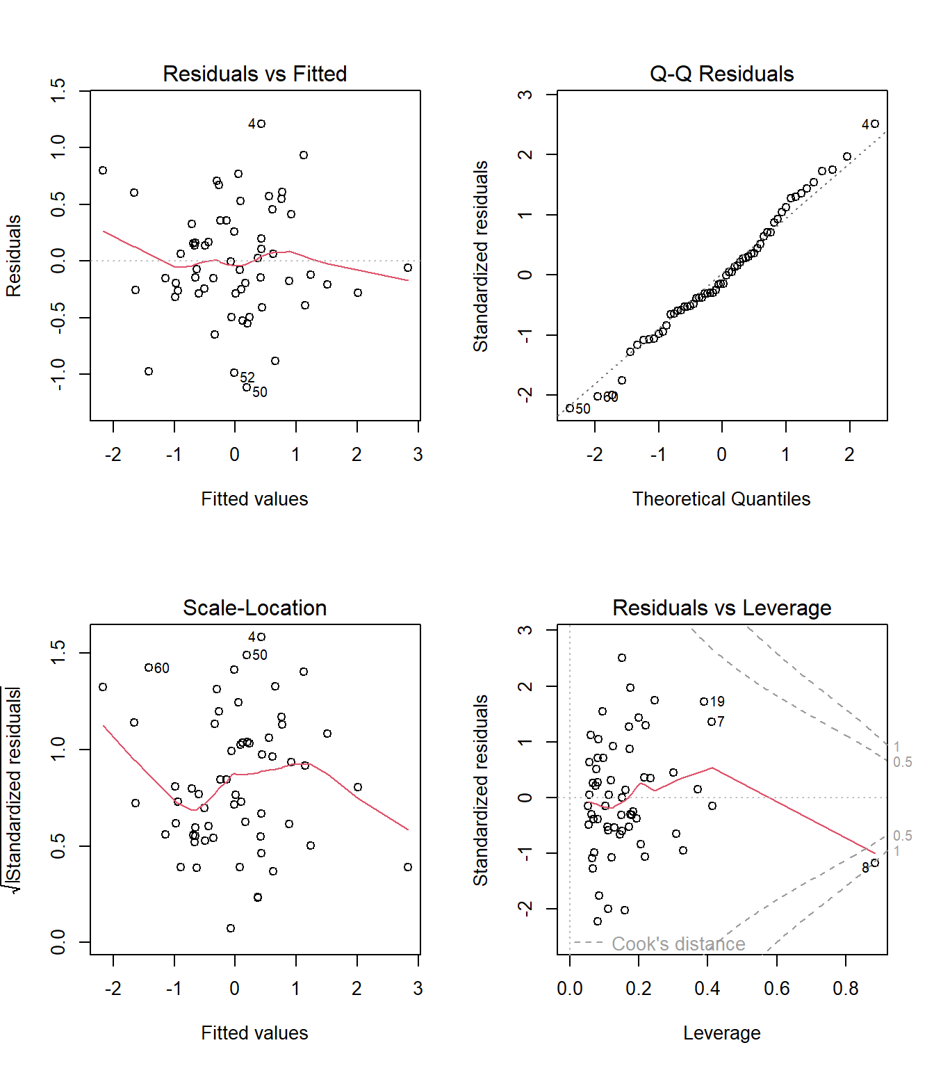

We now seem to have a point with a pretty substantial Cook’s distance, specifically the point from row 8 of the data.

pollution |> slice(8) |> select(x1:x12)

# A tibble: 1 × 12
     x1    x2    x3    x4    x5    x6    x7    x8    x9   x10   x11   x12
  <dbl> <dbl> <dbl> <dbl> <dbl> <dbl> <dbl> <dbl> <dbl> <dbl> <dbl> <dbl>
1    11    53    68   9.2  2.99  12.1  90.6    47   7.8  48.9  12.3   648

pollution |> slice(8) |> select(x13:x15, y, y_inverse, out_std)

# A tibble: 1 × 6
    x13   x14   x15     y y_inverse out_std[,1]
  <dbl> <dbl> <dbl> <dbl>     <dbl>       <dbl>
1   319   130    47  862.   0.00116        1.30

So what is unusual about Row 8? Well, it has an especially large value of x12 compared to the rest of the data.

describe(pollution$x12)

pollution$x12 
       n  missing distinct     Info     Mean      Gmd      .05      .10 
      60        0       34    0.998    37.85    52.03     3.95     5.00 
     .25      .50      .75      .90      .95 
    7.00    14.50    30.25    56.90   106.95 

lowest :   1   3   4   5   6, highest:  88 105 144 311 648

That might be part of the problem, especially since stepwise regression maintains variable x12 whereas our LASSO-inspired model (mod_3) does not.