27 Modeling an Ordinal Categorical Outcome

27.1 R Setup Used Here

knitr::opts_chunk$set(comment = NA)

library(broom)
library(gmodels)
library(MASS)
library(nnet)
library(rms)
library(tidyverse) 

theme_set(theme_bw())

27.1.1 Data Load

smart_oh <- readRDS("data/smart_ohio.Rds")

27.2 A subset of the Ohio SMART data

Let’s consider the following data, which uses part of the smart_oh data we built in Chapter 6. The outcome we’ll study now is genhealth, which has five ordered categories. I’ll include the subset of all observations in smart_oh with complete data on these 7 variables.

Variable	Description
`SEQNO`	Subject identification code
`genhealth`	Five categories (1 = Excellent, 2 = Very Good, 3 = Good, 4 = Fair, 5 = Poor) on general health
`physhealth`	Now thinking about your physical health, which includes physical illness and injury, for how many days during the past 30 days was your physical health not good?
`veg_day`	mean number of vegetable servings consumed per day
`costprob`	1 indicates Yes to “Was there a time in the past 12 months when you needed to see a doctor but could not because of cost?”, and 0 otherwise.
`incomegroup`	8 income groups from < 10,000 to 75,000 or more
`bmi`	body-mass index

To make my life easier later, I’m going to drop any subjects with missing data on these variables. I’m also going to drop the subjects who have no missing data, but have a listed bmi above 60.

sm1 <- smart_oh |>
    select(SEQNO, genhealth, physhealth, costprob, veg_day,
           incomegroup, bmi) |>
    filter(bmi <= 60) |>
    drop_na()

In total, we have 5394 subjects in the sm1 sample.

27.2.1 Several Ways of Storing Multi-Categorical data

We will store the information in our outcome, genhealth in both a numeric form (gen_n) and an ordered factor (gen_h) with some abbreviated labels) because we’ll have some use for each approach in this material.

sm1 <- sm1 |>
    mutate(genh = fct_recode(genhealth,
                             "1-E" = "1_Excellent",
                             "2_VG" = "2_VeryGood",
                             "3_G" = "3_Good",
                             "4_F" = "4_Fair",
                             "5_P" = "5_Poor"),
           genh = factor(genh, ordered = TRUE),
           gen_n = as.numeric(genhealth))

sm1 |> count(genh, gen_n, genhealth)

# A tibble: 5 × 4
  genh  gen_n genhealth       n
  <ord> <dbl> <fct>       <int>
1 1-E       1 1_Excellent   822
2 2_VG      2 2_VeryGood   1805
3 3_G       3 3_Good       1667
4 4_F       4 4_Fair        801
5 5_P       5 5_Poor        299

27.3 Building Cross-Tabulations

Is income group associated with general health?

27.3.1 Using base `table` functions

addmargins(table(sm1$incomegroup, sm1$genh))

        
          1-E 2_VG  3_G  4_F  5_P  Sum
  0-9K     14   45   60   74   40  233
  10-14K   12   41   66   93   46  258
  15-19K   40   76  119   96   61  392
  20-24K   51  129  175  100   50  505
  25-34K   51  172  215  123   36  597
  35-49K   97  270  303  118   24  812
  50-74K  128  337  265   94   16  840
  75K+    429  735  464  103   26 1757
  Sum     822 1805 1667  801  299 5394

More people answer Very Good and Good than choose the other categories. It might be easier to look at percentages here.

27.3.1.1 Adding percentages within each row

Here are the percentages giving each genhealth response within each income group.

addmargins(
    round(100*prop.table(
        table(sm1$incomegroup, sm1$genh)
        ,1)
        ,1)
    )

        
           1-E  2_VG   3_G   4_F   5_P   Sum
  0-9K     6.0  19.3  25.8  31.8  17.2 100.1
  10-14K   4.7  15.9  25.6  36.0  17.8 100.0
  15-19K  10.2  19.4  30.4  24.5  15.6 100.1
  20-24K  10.1  25.5  34.7  19.8   9.9 100.0
  25-34K   8.5  28.8  36.0  20.6   6.0  99.9
  35-49K  11.9  33.3  37.3  14.5   3.0 100.0
  50-74K  15.2  40.1  31.5  11.2   1.9  99.9
  75K+    24.4  41.8  26.4   5.9   1.5 100.0
  Sum     91.0 224.1 247.7 164.3  72.9 800.0

So, for example, 11.3% of the genhealth responses in subjects with incomes between 25 and 34 thousand dollars were Excellent.

27.3.1.2 Adding percentages within each column

Here are the percentages in each incomegroup within each genhealth response.

addmargins(
    round(100*prop.table(
        table(sm1$incomegroup, sm1$genh)
        ,2)
        ,1)
    )

        
           1-E  2_VG   3_G   4_F   5_P   Sum
  0-9K     1.7   2.5   3.6   9.2  13.4  30.4
  10-14K   1.5   2.3   4.0  11.6  15.4  34.8
  15-19K   4.9   4.2   7.1  12.0  20.4  48.6
  20-24K   6.2   7.1  10.5  12.5  16.7  53.0
  25-34K   6.2   9.5  12.9  15.4  12.0  56.0
  35-49K  11.8  15.0  18.2  14.7   8.0  67.7
  50-74K  15.6  18.7  15.9  11.7   5.4  67.3
  75K+    52.2  40.7  27.8  12.9   8.7 142.3
  Sum    100.1 100.0 100.0 100.0 100.0 500.1

From this table, we see that 7.4% of the Excellent genhealth responses were given by people with incomes between 25 and 34 thousand dollars.

27.3.2 Using `xtabs`

The xtabs function provides a formula method for obtaining cross-tabulations.

xtabs(~ incomegroup + genh, data = sm1)

           genh
incomegroup 1-E 2_VG 3_G 4_F 5_P
     0-9K    14   45  60  74  40
     10-14K  12   41  66  93  46
     15-19K  40   76 119  96  61
     20-24K  51  129 175 100  50
     25-34K  51  172 215 123  36
     35-49K  97  270 303 118  24
     50-74K 128  337 265  94  16
     75K+   429  735 464 103  26

27.3.3 Storing a table in a tibble

We can store the elements of a cross-tabulation in a tibble, like this:

(sm1.tableA <- sm1 |> count(incomegroup, genh))

# A tibble: 40 × 3
   incomegroup genh      n
   <fct>       <ord> <int>
 1 0-9K        1-E      14
 2 0-9K        2_VG     45
 3 0-9K        3_G      60
 4 0-9K        4_F      74
 5 0-9K        5_P      40
 6 10-14K      1-E      12
 7 10-14K      2_VG     41
 8 10-14K      3_G      66
 9 10-14K      4_F      93
10 10-14K      5_P      46
# ℹ 30 more rows

From such a tibble, we can visualize the data in many ways, but we can also return to xtabs and include the frequencies (n) in that setup.

xtabs(n ~ incomegroup + genh, data = sm1.tableA)

           genh
incomegroup 1-E 2_VG 3_G 4_F 5_P
     0-9K    14   45  60  74  40
     10-14K  12   41  66  93  46
     15-19K  40   76 119  96  61
     20-24K  51  129 175 100  50
     25-34K  51  172 215 123  36
     35-49K  97  270 303 118  24
     50-74K 128  337 265  94  16
     75K+   429  735 464 103  26

And, we can get the \(\chi^2\) test of independence, with:

summary(xtabs(n ~ incomegroup + genh, data = sm1.tableA))

Call: xtabs(formula = n ~ incomegroup + genh, data = sm1.tableA)
Number of cases in table: 5394 
Number of factors: 2 
Test for independence of all factors:
    Chisq = 894.2, df = 28, p-value = 3.216e-170

27.3.4 Using `CrossTable` from the `gmodels` package

The CrossTable function from the gmodels package produces a cross-tabulation with various counts and proportions like people often generate with SPSS and SAS.

CrossTable(sm1$incomegroup, sm1$genh, chisq = T)


 
   Cell Contents
|-------------------------|
|                       N |
| Chi-square contribution |
|           N / Row Total |
|           N / Col Total |
|         N / Table Total |
|-------------------------|

 
Total Observations in Table:  5394 

 
                | sm1$genh 
sm1$incomegroup |       1-E |      2_VG |       3_G |       4_F |       5_P | Row Total | 
----------------|-----------|-----------|-----------|-----------|-----------|-----------|
           0-9K |        14 |        45 |        60 |        74 |        40 |       233 | 
                |    13.027 |    13.941 |     2.002 |    44.865 |    56.796 |           | 
                |     0.060 |     0.193 |     0.258 |     0.318 |     0.172 |     0.043 | 
                |     0.017 |     0.025 |     0.036 |     0.092 |     0.134 |           | 
                |     0.003 |     0.008 |     0.011 |     0.014 |     0.007 |           | 
----------------|-----------|-----------|-----------|-----------|-----------|-----------|
         10-14K |        12 |        41 |        66 |        93 |        46 |       258 | 
                |    18.980 |    23.806 |     2.366 |    78.061 |    70.259 |           | 
                |     0.047 |     0.159 |     0.256 |     0.360 |     0.178 |     0.048 | 
                |     0.015 |     0.023 |     0.040 |     0.116 |     0.154 |           | 
                |     0.002 |     0.008 |     0.012 |     0.017 |     0.009 |           | 
----------------|-----------|-----------|-----------|-----------|-----------|-----------|
         15-19K |        40 |        76 |       119 |        96 |        61 |       392 | 
                |     6.521 |    23.208 |     0.038 |    24.531 |    70.973 |           | 
                |     0.102 |     0.194 |     0.304 |     0.245 |     0.156 |     0.073 | 
                |     0.049 |     0.042 |     0.071 |     0.120 |     0.204 |           | 
                |     0.007 |     0.014 |     0.022 |     0.018 |     0.011 |           | 
----------------|-----------|-----------|-----------|-----------|-----------|-----------|
         20-24K |        51 |       129 |       175 |       100 |        50 |       505 | 
                |     8.756 |     9.463 |     2.296 |     8.340 |    17.301 |           | 
                |     0.101 |     0.255 |     0.347 |     0.198 |     0.099 |     0.094 | 
                |     0.062 |     0.071 |     0.105 |     0.125 |     0.167 |           | 
                |     0.009 |     0.024 |     0.032 |     0.019 |     0.009 |           | 
----------------|-----------|-----------|-----------|-----------|-----------|-----------|
         25-34K |        51 |       172 |       215 |       123 |        36 |       597 | 
                |    17.567 |     3.862 |     5.042 |    13.307 |     0.255 |           | 
                |     0.085 |     0.288 |     0.360 |     0.206 |     0.060 |     0.111 | 
                |     0.062 |     0.095 |     0.129 |     0.154 |     0.120 |           | 
                |     0.009 |     0.032 |     0.040 |     0.023 |     0.007 |           | 
----------------|-----------|-----------|-----------|-----------|-----------|-----------|
         35-49K |        97 |       270 |       303 |       118 |        24 |       812 | 
                |     5.779 |     0.011 |    10.798 |     0.055 |     9.808 |           | 
                |     0.119 |     0.333 |     0.373 |     0.145 |     0.030 |     0.151 | 
                |     0.118 |     0.150 |     0.182 |     0.147 |     0.080 |           | 
                |     0.018 |     0.050 |     0.056 |     0.022 |     0.004 |           | 
----------------|-----------|-----------|-----------|-----------|-----------|-----------|
         50-74K |       128 |       337 |       265 |        94 |        16 |       840 | 
                |     0.000 |    11.121 |     0.112 |     7.575 |    20.061 |           | 
                |     0.152 |     0.401 |     0.315 |     0.112 |     0.019 |     0.156 | 
                |     0.156 |     0.187 |     0.159 |     0.117 |     0.054 |           | 
                |     0.024 |     0.062 |     0.049 |     0.017 |     0.003 |           | 
----------------|-----------|-----------|-----------|-----------|-----------|-----------|
           75K+ |       429 |       735 |       464 |       103 |        26 |      1757 | 
                |    97.108 |    36.780 |    11.492 |    95.573 |    52.335 |           | 
                |     0.244 |     0.418 |     0.264 |     0.059 |     0.015 |     0.326 | 
                |     0.522 |     0.407 |     0.278 |     0.129 |     0.087 |           | 
                |     0.080 |     0.136 |     0.086 |     0.019 |     0.005 |           | 
----------------|-----------|-----------|-----------|-----------|-----------|-----------|
   Column Total |       822 |      1805 |      1667 |       801 |       299 |      5394 | 
                |     0.152 |     0.335 |     0.309 |     0.148 |     0.055 |           | 
----------------|-----------|-----------|-----------|-----------|-----------|-----------|

 
Statistics for All Table Factors


Pearson's Chi-squared test 
------------------------------------------------------------
Chi^2 =  894.1685     d.f. =  28     p =  3.216132e-170

27.4 Graphing Categorical Data

27.4.1 A Bar Chart for a Single Variable

ggplot(sm1, aes(x = genhealth, fill = genhealth)) + 
    geom_bar() +
    scale_fill_brewer(palette = "Set1") +
    guides(fill = "none")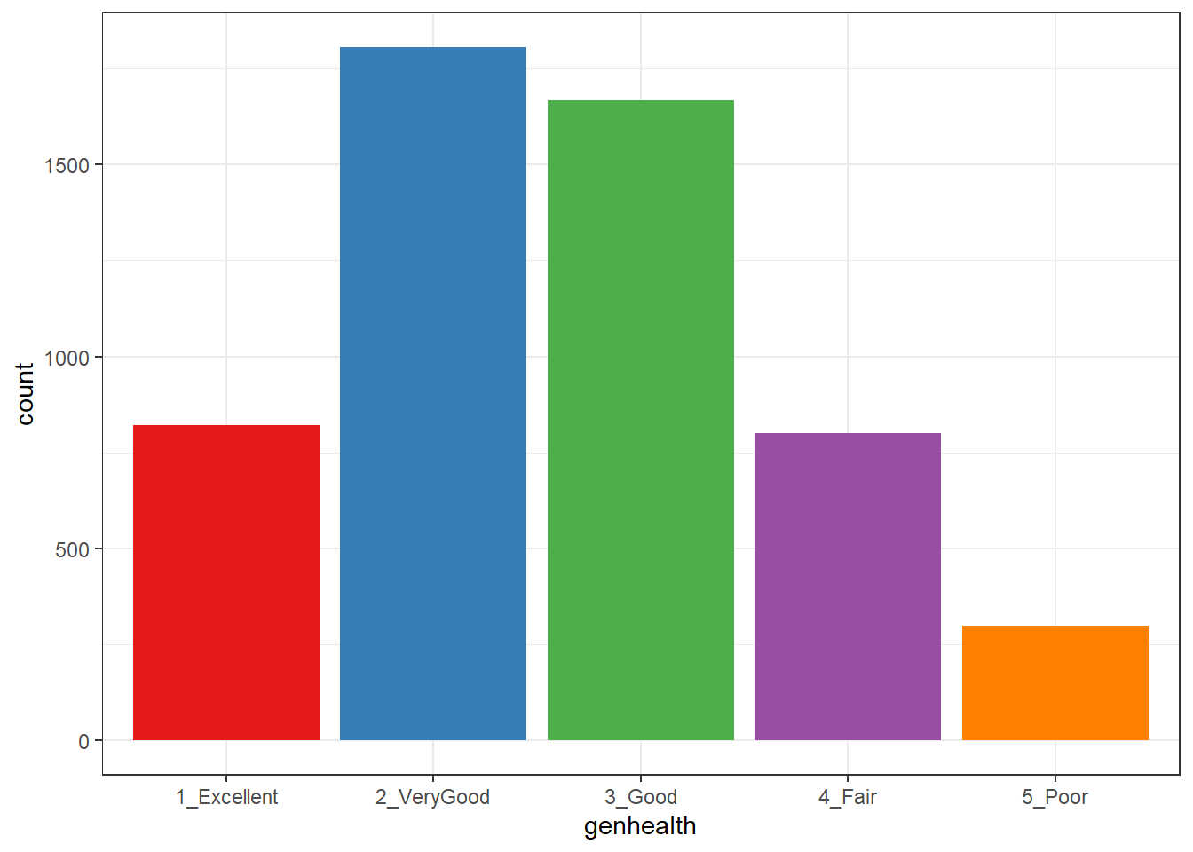

or, you might prefer to plot percentages, perhaps like this:

ggplot(sm1, aes(x = genhealth, fill = genhealth)) + 
    geom_bar(aes(y = (..count..)/sum(..count..))) +
    geom_text(aes(y = (..count..)/sum(..count..), 
                  label = scales::percent((..count..) / 
                                        sum(..count..))),
              stat = "count", vjust = 1, 
              color = "white", size = 5) +
    scale_y_continuous(labels = scales::percent) +
    scale_fill_brewer(palette = "Dark2") +
    guides(fill = "none") + 
    labs(y = "Percentage")

Warning: The dot-dot notation (`..count..`) was deprecated in ggplot2 3.4.0.
ℹ Please use `after_stat(count)` instead.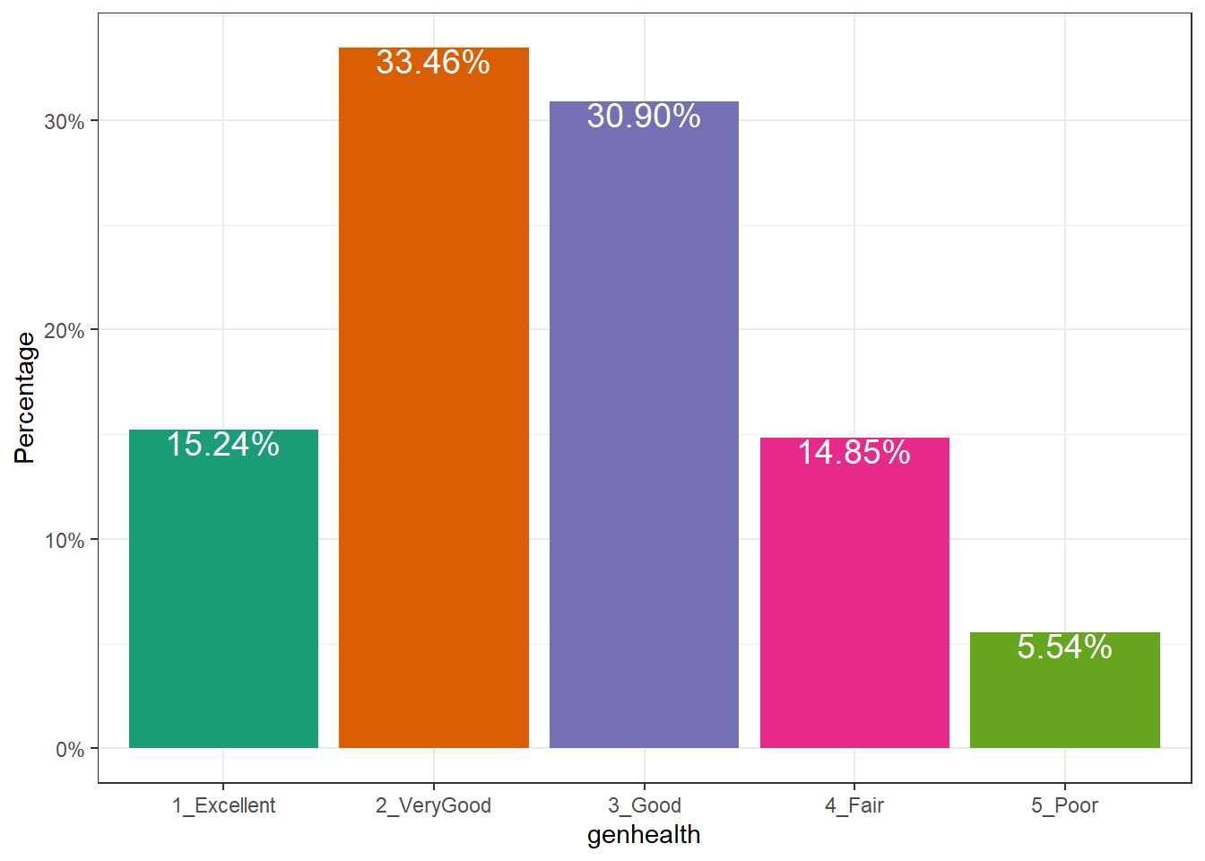

Use bar charts, rather than pie charts.

27.4.2 A Counts Chart for a 2-Way Cross-Tabulation

ggplot(sm1, aes(x = genhealth, y = incomegroup)) + 
    geom_count()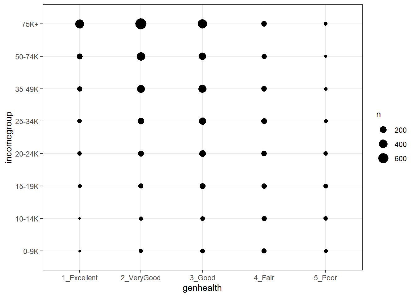

27.5 Building a Model for `genh` using `veg_day`

To begin, we’ll predict each subject’s genh response using just one predictor, veg_day.

27.5.1 A little EDA

Let’s start with a quick table of summary statistics.

sm1 |> group_by(genh) |>
    summarize(n(), mean(veg_day), sd(veg_day), median(veg_day))

# A tibble: 5 × 5
  genh  `n()` `mean(veg_day)` `sd(veg_day)` `median(veg_day)`
  <ord> <int>           <dbl>         <dbl>             <dbl>
1 1-E     822            2.16          1.46              1.87
2 2_VG   1805            1.99          1.13              1.78
3 3_G    1667            1.86          1.11              1.71
4 4_F     801            1.74          1.18              1.57
5 5_P     299            1.71          1.06              1.57

To actually see what’s going on, we might build a comparison boxplot, or violin plot. The plot below shows both, together, with the violin plot helping to indicate the skewed nature of the veg_day data and the boxplot indicating quartiles and outlying values within each genhealth category.

ggplot(sm1, aes(x = genhealth, y = veg_day)) +
    geom_violin(aes(fill = genhealth), trim = TRUE) +
    geom_boxplot(width = 0.2) +
    guides(fill = "none", color = "none") +
    theme_bw()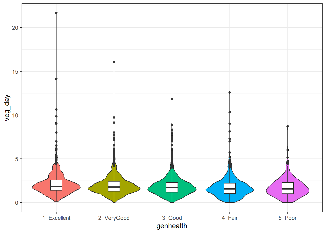

27.5.2 Describing the Proportional-Odds Cumulative Logit Model

To fit the ordinal logistic regression model (specifically, a proportional-odds cumulative-logit model) in this situation, we’ll use the polr function in the MASS package.

Our outcome is genh, which has five ordered levels, with 1-E best and 5-P worst.
Our model will include one quantitative predictor, veg_day.

The model will have four logit equations:

one estimating the log odds that genh will be less than or equal to 1 (i.e. genhealth = 1_Excellent,)
one estimating the log odds that genh \(\leq\) 2 (i.e. genhealth = 1_Excellent or 2_VeryGood,)
another estimating the log odds that genh \(\leq\) 3 (i.e. genhealth = 1_Excellent, 2_VeryGood or 3_Good,) and, finally,
one estimating the log odds that genh \(\leq\) 4 (i.e. genhealth = 1_Excellent, 2_VeryGood, 3_Good or 4_Fair)

That’s all we need to estimate the five categories, since Pr(genh \(\leq\) 5) = 1, because (5_Poor) is the maximum category for genhealth.

We’ll have a total of five free parameters when we add in the slope for veg_day, and I’ll label these parameters as \(\zeta_1, \zeta_2, \zeta_3, \zeta_4\) and \(\beta_1\). The \(\zeta\)s are read as “zeta” values, and the people who built the polr function use that term.

The four logistic equations that will be fit differ only by their intercepts. They are:

\[ logit[Pr(genh \leq 1)] = log \frac{Pr(genh \leq 1}{Pr(genh > 1)} = \zeta_1 - \beta_1 veg_day \]

which describes the log odds of a genh value of 1 (Excellent) as compared to a genh value greater than 1 (which includes Very Good, Good, Fair and Poor).

The second logit model is:

\[ logit[Pr(genh \leq 2)] = log \frac{Pr(genh \leq 2}{Pr(genh > 2)} = \zeta_2 - \beta_1 veg_day \]

which describes the log odds of a genh value of 1 (Excellent) or 2 (Very Good) as compared to a genh value greater than 2 (which includes Good, Fair and Poor).

Next we have:

\[ logit[Pr(genh \leq 3)] = log \frac{Pr(genh \leq 3}{Pr(genh > 3)} = \zeta_3 - \beta_1 veg_day \]

which describes the log odds of a genh value of 1 (Excellent) or 2 (Very Good) or 3 (Good) as compared to a genh value greater than 3 (which includes Fair and Poor).

Finally, we have

\[ logit[Pr(genh \leq 4)] = log \frac{Pr(genh \leq 4}{Pr(genh > 4)} = \zeta_4 - \beta_1 veg_day \]

which describes the log odds of a genh value of 4 or less, which includes Excellent, Very Good, Good and Fair as compared to a genh value greater than 4 (which is Poor).

Again, the intercept term is the only piece that varies across the four equations.

In this case, a positive coefficient \(\beta_1\) for veg_day means that increasing the value of veg_day would increase the genh category (describing a worse level of general health, since higher values of genh are associated with worse health.)

27.5.3 Fitting a Proportional Odds Logistic Regression with `polr`

Our model m1 will use proportional odds logistic regression (sometimes called an ordered logit model) to predict genh on the basis of veg_day. The polr function from the MASS package will be our main tool. Note that we include Hess = TRUE to retain what is called the Hessian matrix, which lets R calculate standard errors more effectively in summary and other follow-up descriptions of the model.

m1 <- polr(genh ~ veg_day, 
            data = sm1, Hess = TRUE)

summary(m1)

Call:
polr(formula = genh ~ veg_day, data = sm1, Hess = TRUE)

Coefficients:
          Value Std. Error t value
veg_day -0.1847    0.02178   -8.48

Intercepts:
         Value    Std. Error t value 
1-E|2_VG  -2.0866   0.0584   -35.7590
2_VG|3_G  -0.4065   0.0498    -8.1621
3_G|4_F    1.0202   0.0521    19.5771
4_F|5_P    2.5002   0.0710    35.2163

Residual Deviance: 15669.85 
AIC: 15679.85

confint(m1)

Waiting for profiling to be done...

     2.5 %     97.5 % 
-0.2277073 -0.1423088

27.6 Interpreting Model `m1`

27.6.1 Looking at Predictions

Consider two individuals:

Harry, who eats an average of 2.0 servings of vegetables per day, so Harry’s veg_day = 2, and
Sally, who eats an average of 1.0 serving of vegetables per day, so Sally’s veg_day = 1.

We’re going to start by using our model m1 to predict the genh for Harry and Sally, so we can see the effect (on the predicted genh probabilities) of a change of one unit in veg_day.

For example, what are the log odds that Harry, with veg_day = 2, will describe his genh as Excellent (genh \(\leq\) 1)?

\[ logit[Pr(genh \leq 1)] = \zeta_1 - \beta_1 veg\_day \]

\[ logit[Pr(genh \leq 1)] = -2.0866 - (-0.1847) veg\_day \]

\[ logit[Pr(genh \leq 1)] = -2.0866 - (-0.1847) (2) = -1.7172 \]

That’s not much help. So we’ll convert it to a probability by taking the inverse logit. The formula is

\[ Pr(genh \leq 1) = \frac{exp(\zeta_1 + \beta_1 veg_day)}{1 + exp(\zeta_1 + \beta_1 veg_day)} = \frac{exp(-1.7172)}{1 + exp(-1.7172)} = \frac{0.180}{1.180} = 0.15 \]

So the model estimates a 15% probability that Harry will describe his genh as Excellent.

OK. Now, what are the log odds that Harry, who eats 2 servings per day, will describe his genh as either Excellent or Very Good (genh \(\leq\) 2)?

\[ logit[Pr(genh \leq 2)] = \zeta_2 - \beta_1 veg\_day \]

\[ logit[Pr(genh \leq 2)] = -0.4065 - (-0.1847) veg\_day \\ \]

\[ logit[Pr(genh \leq 2)] = -0.4065 - (-0.1847) (2) = -0.0371 \]

Again, we’ll convert this to a probability by taking the inverse logit.

\[ Pr(genh \leq 2) = \frac{exp(\zeta_2 + \beta_1 veg_day)}{1 + exp(\zeta_2 + \beta_1 veg_day)} = \frac{exp(-0.0371)}{1 + exp(-0.0371)} = \frac{0.964}{1.964} = 0.49 \]

So, the model estimates a probability of .49 that Harry will describe his genh as either Excellent or Very Good, so by subtraction, that’s a probability of .34 that Harry describes his genh as Very Good.

Happily, that’s the last time we’ll calculate this by hand.

27.6.2 Making Predictions for Harry (and Sally) with `predict`

Suppose Harry eats 2 servings of vegetables per day on average, and Sally eats 1.

temp.dat <- data.frame(name = c("Harry", "Sally"), 
                       veg_day = c(2,1))

predict(m1, temp.dat, type = "p")

        1-E      2_VG       3_G       4_F        5_P
1 0.1522351 0.3385119 0.3097906 0.1457864 0.05367596
2 0.1298931 0.3148971 0.3246105 0.1667285 0.06387071

The predicted probabilities of falling into each category of genh are:

Subject	`veg_day`	Pr(1_E)	Pr(2_VG)	Pr(3_G)	Pr(4_F)	Pr(5_P)
Harry	2	15.2	33.9	31.0	14.6	5.4
Sally	1	13.0	31.4	32.5	16.7	6.4

Harry has a higher predicted probability of lower (healthier) values of genh. Specifically, Harry has a higher predicted probability than Sally of falling into the Excellent and Very Good categories, and a lower probability than Sally of falling into the Good, Fair and Poor categories.
This means that Harry, with a higher veg_day is predicted to have, on average, a lower (that is to say, healthier) value of genh.
As we’ll see, this association will be indicated by a negative coefficient of veg_day in the proportional odds logistic regression model.

27.6.3 Predicting the actual classification of `genh`

The default prediction approach actually returns the predicted genh classification for Harry and Sally, which is just the classification with the largest predicted probability. Here, for Harry that is Very Good, and for Sally, that’s Good.

predict(m1, temp.dat)

[1] 2_VG 3_G 
Levels: 1-E 2_VG 3_G 4_F 5_P

27.6.4 A Cross-Tabulation of Predictions?

addmargins(table(predict(m1), sm1$genh))

      
        1-E 2_VG  3_G  4_F  5_P  Sum
  1-E     6    3    3    3    0   15
  2_VG  647 1398 1198  525  192 3960
  3_G   169  404  466  273  107 1419
  4_F     0    0    0    0    0    0
  5_P     0    0    0    0    0    0
  Sum   822 1805 1667  801  299 5394

The m1 model classifies all subjects in the sm1 sample as either Excellent, Very Good or Good, and most subjects as Very Good or Good.

27.6.5 The Fitted Model Equations

summary(m1)

Call:
polr(formula = genh ~ veg_day, data = sm1, Hess = TRUE)

Coefficients:
          Value Std. Error t value
veg_day -0.1847    0.02178   -8.48

Intercepts:
         Value    Std. Error t value 
1-E|2_VG  -2.0866   0.0584   -35.7590
2_VG|3_G  -0.4065   0.0498    -8.1621
3_G|4_F    1.0202   0.0521    19.5771
4_F|5_P    2.5002   0.0710    35.2163

Residual Deviance: 15669.85 
AIC: 15679.85

The first part of the output provides coefficient estimates for the veg_day predictor, and these are followed by the estimates for the various model intercepts. Plugging in the estimates, we have:

\[ logit[Pr(genh \leq 1)] = -2.0866 - (-0.1847) veg_day \]

\[ logit[Pr(genh \leq 2)] = -0.4065 - (-0.1847) veg_day \]

\[ logit[Pr(genh \leq 3)] = 1.0202 - (-0.1847) veg_day \]

\[ logit[Pr(genh \leq 4)] = 2.5002 - (-0.1847) veg_day \]

Note that we can obtain these pieces separately as follows:

m1$zeta

  1-E|2_VG   2_VG|3_G    3_G|4_F    4_F|5_P 
-2.0866313 -0.4064704  1.0202035  2.5001655

shows the boundary intercepts, and

m1$coefficients

   veg_day 
-0.1847272

shows the regression coefficient for veg_day.

27.6.6 Interpreting the `veg_day` coefficient

The first part of the output provides coefficient estimates for the veg_day predictor.

The estimated slope for veg_day is -0.1847
- Remember Harry and Sally, who have the same values of bmi and costprob, but Harry eats one more serving than Sally does. We noted that Harry is predicted by the model to have a smaller (i.e. healthier) genh response than Sally.
- So a negative coefficient here means that higher values of veg_day are associated with more of the probability distribution falling in lower values of genh.
- We usually don’t interpret this slope (on the log odds scale) directly, but rather exponentiate it.

27.6.7 Exponentiating the Slope Coefficient to facilitate Interpretation

We can compute the odds ratio associated with veg_day and its confidence interval as follows…

exp(coef(m1))

  veg_day 
0.8313311

exp(confint(m1))

Waiting for profiling to be done...

    2.5 %    97.5 % 
0.7963573 0.8673534

So, if Harry eats one more serving of vegetables than Sally, our model predicts that Harry will have 83.1% of the odds of Sally of having a larger genh score. That means that Harry is likelier to have a smaller genh score.
- Since genh gets larger as a person’s general health gets worse (moves from Excellent towards Poor), this means that since Harry is predicted to have smaller odds of a larger genh score, he is also predicted to have smaller odds of worse general health.
- Our 95% confidence interval around that estimated odds ratio of 0.831 is (0.796, 0.867). Since that interval is entirely below 1, the odds of having the larger (worse) genh for Harry are detectably lower than the odds for Sally.
- So, an increase in veg_day is associated with smaller (better) genh scores.

27.6.8 Comparison to a Null Model

We can fit a model with intercepts only to assess the predictive value of veg_day in our model m1, using the anova function.

m0 <- polr(genh ~ 1, data = sm1)

anova(m1, m0)

Likelihood ratio tests of ordinal regression models

Response: genh
    Model Resid. df Resid. Dev   Test    Df LR stat. Pr(Chi)
1       1      5390   15744.89                              
2 veg_day      5389   15669.85 1 vs 2     1 75.04297       0

We could also compare model m1 to the null model m0 with AIC or BIC.

AIC(m1, m0)

   df      AIC
m1  5 15679.85
m0  4 15752.89

BIC(m1,m0)

   df      BIC
m1  5 15712.81
m0  4 15779.26

Model m1 looks like the better choice so far.

27.7 The Assumption of Proportional Odds

Let us calculate the odds for all levels of genh if a person eats two servings of vegetables. First, we’ll get the probabilities, in another way, to demonstrate how to do so…

(prob.2 <- exp(m1$zeta - 2*m1$coefficients)/(1 + exp(m1$zeta - 2*m1$coefficients)))

 1-E|2_VG  2_VG|3_G   3_G|4_F   4_F|5_P 
0.1522351 0.4907471 0.8005376 0.9463240

(prob.1 <- exp(m1$zeta - 1*m1$coefficients)/(1 + exp(m1$zeta - 1*m1$coefficients)))

 1-E|2_VG  2_VG|3_G   3_G|4_F   4_F|5_P 
0.1298931 0.4447902 0.7694008 0.9361293

Now, we’ll calculate the odds, first for a subject eating two servings:

(odds.2 = prob.2/(1-prob.2))

  1-E|2_VG   2_VG|3_G    3_G|4_F    4_F|5_P 
 0.1795724  0.9636607  4.0134766 17.6303153

And here are the odds, for a subject eating one serving per day:

(odds.1 = prob.1/(1-prob.1))

  1-E|2_VG   2_VG|3_G    3_G|4_F    4_F|5_P 
 0.1492841  0.8011211  3.3365277 14.6566285

Now, let’s take the ratio of the odds for someone who eats two servings over the odds for someone who eats one.

odds.2/odds.1

1-E|2_VG 2_VG|3_G  3_G|4_F  4_F|5_P 
 1.20289  1.20289  1.20289  1.20289

They are all the same. The odds ratios are equal, which means they are proportional. For any level of genh, the estimated odds that a person who eats 2 servings has better (lower) genh is about 1.2 times the odds for someone who eats one serving. Those who eat more vegetables have higher odds of better (lower) genh. Less than 1 means lower odds, and more than 1 means greater odds.

Now, let’s take the log of the odds ratios:

log(odds.2/odds.1)

 1-E|2_VG  2_VG|3_G   3_G|4_F   4_F|5_P 
0.1847272 0.1847272 0.1847272 0.1847272

That should be familiar. It is the slope coefficient in the model summary, without the minus sign. R tacks on a minus sign so that higher levels of predictors correspond to the ordinal outcome falling in the higher end of its scale.

If we exponentiate the slope estimated by R (-0.1847), we get 0.83. If we have two people, and A eats one more serving of vegetables on average than B, then the estimated odds of A having a higher ‘genh’ (i.e. worse general health) are 83% as high as B’s.

27.7.1 Testing the Proportional Odds Assumption

One way to test the proportional odds assumption is to compare the fit of the proportional odds logistic regression to a model that does not make that assumption. A natural candidate is a multinomial logit model, which is typically used to model unordered multi-categorical outcomes, and fits a slope to each level of the genh outcome in this case, as opposed to the proportional odds logit, which fits only one slope across all levels.

Since the proportional odds logistic regression model is nested in the multinomial logit, we can perform a likelihood ratio test. To do this, we first fit the multinomial logit model, with the multinom function from the nnet package.

(m1_multi <- multinom(genh ~ veg_day, data = sm1))

# weights:  15 (8 variable)
initial  value 8681.308100 
iter  10 value 7890.985276
final  value 7835.248471 
converged

Call:
multinom(formula = genh ~ veg_day, data = sm1)

Coefficients:
     (Intercept)     veg_day
2_VG   0.9791063 -0.09296694
3_G    1.0911990 -0.19260067
4_F    0.5708594 -0.31080687
5_P   -0.3583310 -0.34340619

Residual Deviance: 15670.5 
AIC: 15686.5

The multinomial logit fits four intercepts and four slopes, for a total of 8 estimated parameters. The proportional odds logit, as we’ve seen, fits four intercepts and one slope, for a total of 5. The difference is 3, and we use that number in the sequence below to build our test of the proportional odds assumption.

LL_1 <- logLik(m1)
LL_1m <- logLik(m1_multi)
(G <- -2 * (LL_1[1] - LL_1m[1]))

[1] -0.6488392

pchisq(G, 3, lower.tail = FALSE)

[1] 1

The p value is very large, so it indicates that the proportional odds model fits about as well as the more complex multinomial logit. A large p value here isn’t always the best way to assess the proportional odds assumption, but it does provide some evidence of model adequacy.

27.8 Can model `m1` be fit using `rms` tools?

Yes.

d <- datadist(sm1)
options(datadist = "d")
m1_lrm <- lrm(genh ~ veg_day, data = sm1, x = T, y = T)

m1_lrm

Logistic Regression Model

lrm(formula = genh ~ veg_day, data = sm1, x = T, y = T)


Frequencies of Responses

 1-E 2_VG  3_G  4_F  5_P 
 822 1805 1667  801  299 

                       Model Likelihood     Discrimination    Rank Discrim.    
                             Ratio Test            Indexes          Indexes    
Obs          5394    LR chi2      75.04     R2       0.015    C       0.555    
max |deriv| 2e-13    d.f.             1    R2(1,5394)0.014    Dxy     0.111    
                     Pr(> chi2) <0.0001    R2(1,4995)0.015    gamma   0.111    
                                            Brier    0.247    tau-a   0.082    

        Coef    S.E.   Wald Z Pr(>|Z|)
y>=2_VG  2.0866 0.0584  35.76 <0.0001 
y>=3_G   0.4065 0.0498   8.16 <0.0001 
y>=4_F  -1.0202 0.0521 -19.58 <0.0001 
y>=5_P  -2.5002 0.0710 -35.22 <0.0001 
veg_day -0.1847 0.0218  -8.48 <0.0001

The model has a small p value (remember the large sample size) but nonetheless appears very weak, with a Nagelkerke \(R^2\) of 0.015, and a C statistic of 0.555.

summary(m1_lrm)

             Effects              Response : genh 

 Factor      Low  High Diff. Effect   S.E.     Lower 0.95 Upper 0.95
 veg_day     1.21 2.36 1.15  -0.21243 0.025051 -0.26153   -0.16334  
  Odds Ratio 1.21 2.36 1.15   0.80861       NA  0.76987    0.84931

A change from 1.21 to 2.36 servings in veg_day is associated with an odds ratio of 0.81, with 95% confidence interval (0.77, 0.85). Since these values are all below 1, we have a clear indication of a statistically detectable effect of veg_day with higher veg_day associated with lower genh, which means, in this case, better health.

There is also a tool in rms called orm which may be used to fit a wide array of ordinal regression models. I suggest you read Frank Harrell’s book on Regression Modeling Strategies if you want to learn more.

27.9 Building a Three-Predictor Model

Now, we’ll model genh using veg_day, bmi and costprob.

27.9.1 Scatterplot Matrix

GGally::ggpairs(sm1 |> 
                    select(bmi, veg_day, costprob, genh))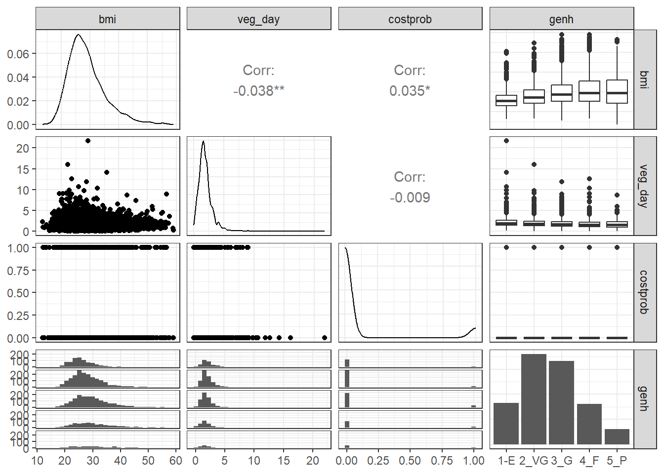

We might choose to plot the costprob data as a binary factor, rather than the raw 0-1 numbers included above, but not at this time.

27.9.2 Our Three-Predictor Model, `m2`

m2 <- polr(genh ~ veg_day + bmi + costprob, data = sm1)

summary(m2)


Re-fitting to get Hessian

Call:
polr(formula = genh ~ veg_day + bmi + costprob, data = sm1)

Coefficients:
            Value Std. Error t value
veg_day  -0.17130   0.021783  -7.864
bmi       0.06673   0.003855  17.311
costprob  0.96825   0.084871  11.409

Intercepts:
         Value   Std. Error t value
1-E|2_VG -0.1252  0.1229    -1.0183
2_VG|3_G  1.6358  0.1234    13.2572
3_G|4_F   3.1534  0.1294    24.3755
4_F|5_P   4.6881  0.1412    33.1928

Residual Deviance: 15229.24 
AIC: 15243.24

This model contains four intercepts (to cover the five genh categories) and three slopes (one each for veg_day, bmi and costprob.)

27.9.3 Does the three-predictor model outperform `m1`?

anova(m1, m2)

Likelihood ratio tests of ordinal regression models

Response: genh
                     Model Resid. df Resid. Dev   Test    Df LR stat. Pr(Chi)
1                  veg_day      5389   15669.85                              
2 veg_day + bmi + costprob      5387   15229.24 1 vs 2     2 440.6041       0

It looks like the fit improves as we move from model 1 to model 2. The AIC and BIC are also better for the three-predictor model than they were for the model with veg_day alone.

AIC(m1, m2)

   df      AIC
m1  5 15679.85
m2  7 15243.24

BIC(m1, m2)

   df      BIC
m1  5 15712.81
m2  7 15289.40

27.9.4 Wald tests for individual predictors

To obtain the appropriate Wald tests, we can use lrm to fit the model instead.

d <- datadist(sm1)
options(datadist = "d")
m2_lrm <- lrm(genh ~ veg_day + bmi + costprob, 
              data = sm1, x = T, y = T)
m2_lrm

Logistic Regression Model

lrm(formula = genh ~ veg_day + bmi + costprob, data = sm1, x = T, 
    y = T)


Frequencies of Responses

 1-E 2_VG  3_G  4_F  5_P 
 822 1805 1667  801  299 

                       Model Likelihood     Discrimination    Rank Discrim.    
                             Ratio Test            Indexes          Indexes    
Obs          5394    LR chi2     515.65     R2       0.096    C       0.629    
max |deriv| 4e-09    d.f.             3    R2(3,5394)0.091    Dxy     0.258    
                     Pr(> chi2) <0.0001    R2(3,4995)0.098    gamma   0.258    
                                            Brier    0.231    tau-a   0.192    

         Coef    S.E.   Wald Z Pr(>|Z|)
y>=2_VG   0.1252 0.1229   1.02 0.3085  
y>=3_G   -1.6358 0.1234 -13.26 <0.0001 
y>=4_F   -3.1534 0.1294 -24.38 <0.0001 
y>=5_P   -4.6881 0.1412 -33.19 <0.0001 
veg_day  -0.1713 0.0218  -7.86 <0.0001 
bmi       0.0667 0.0039  17.31 <0.0001 
costprob  0.9683 0.0849  11.41 <0.0001

It appears that each of the added predictors (bmi and costprob) adds statistically detectable value to the model.

27.9.5 A Cross-Tabulation of Predictions?

addmargins(table(predict(m2), sm1$genh))

      
        1-E 2_VG  3_G  4_F  5_P  Sum
  1-E     6    5    4    1    0   16
  2_VG  686 1295  950  388  141 3460
  3_G   128  495  672  374  135 1804
  4_F     1    9   38   36   20  104
  5_P     1    1    3    2    3   10
  Sum   822 1805 1667  801  299 5394

At least the m2 model predicted that a few of the cases will fall in the Fair and Poor categories, but still, this isn’t impressive.

27.9.6 Interpreting the Effect Sizes

We can do this in two ways:

By exponentiating the polr output, which shows the effect of increasing each predictor by a single unit
- Increasing veg_day by 1 serving while holding the other predictors constant is associated with reducing the odds (by a factor of 0.84 with 95% CI 0.81, 0.88)) of higher values of genh: hence increasing veg_day is associated with increasing the odds of a response indicating better health.
- Increasing bmi by 1 kg/m² while holding the other predictors constant is associated with increasing the odds (by a factor of 1.07 with 95% CI 1.06, 1.08)) of higher values of genh: hence increasing bmi is associated with reducing the odds of a response indicating better health.
- Increasing costprob from 0 to 1 while holding the other predictors constant is associated with an increase (by a factor of 2.63 with 95% CI 2.23, 3.11)) of a higher genh value. Since higher genh values indicate worse health, those with costprob = 1 are modeled to have generally worse health.

exp(coef(m2))

  veg_day       bmi  costprob 
0.8425722 1.0690045 2.6333356

exp(confint(m2))

Waiting for profiling to be done...


Re-fitting to get Hessian

             2.5 %   97.5 %
veg_day  0.8071346 0.879096
bmi      1.0609722 1.077126
costprob 2.2301783 3.110633

Or by looking at the summary provided by lrm, which like all such summaries produced by rms shows the impact of moving from the 25th to the 75th percentile on all continuous predictors.

summary(m2_lrm)

             Effects              Response : genh 

 Factor      Low   High   Diff.  Effect   S.E.     Lower 0.95 Upper 0.95
 veg_day      1.21  2.360 1.1500 -0.19699 0.025051 -0.24609   -0.14789  
  Odds Ratio  1.21  2.360 1.1500  0.82120       NA  0.78185    0.86252  
 bmi         24.33 31.988 7.6575  0.51097 0.029515  0.45312    0.56882  
  Odds Ratio 24.33 31.988 7.6575  1.66690       NA  1.57320    1.76620  
 costprob     0.00  1.000 1.0000  0.96825 0.084871  0.80191    1.13460  
  Odds Ratio  0.00  1.000 1.0000  2.63330       NA  2.22980    3.10990

plot(summary(m2_lrm))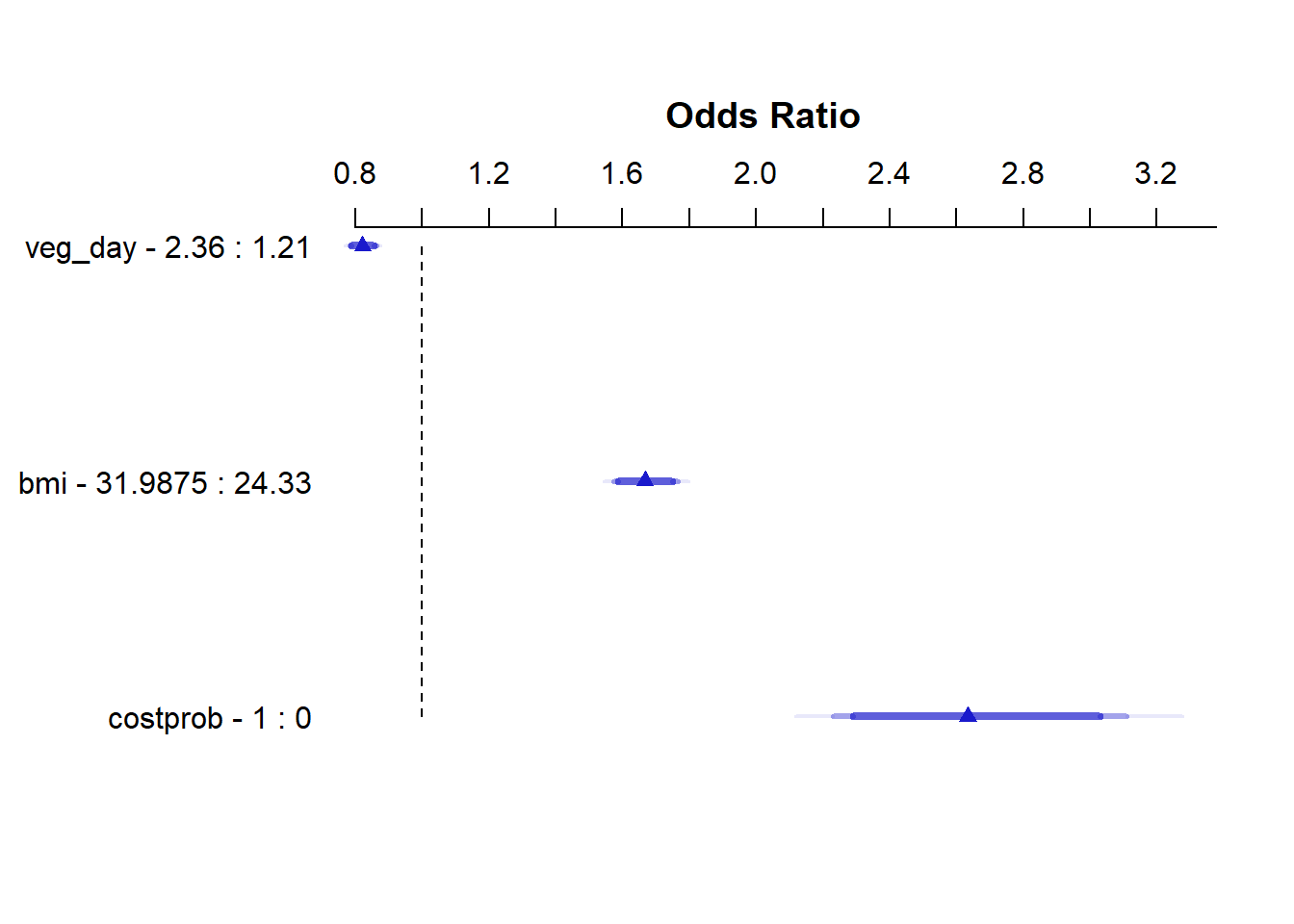

27.9.7 Quality of the Model Fit

Model m2, as we can see from the m2_lrm output, is still weak, with a Nagelkerke \(R^2\) of 0.10, and a C statistic of 0.63.

27.9.8 Validating the Summary Statistics in `m2_lrm`

set.seed(43203); validate(m2_lrm)

          index.orig training    test optimism index.corrected  n
Dxy           0.2583   0.2625  0.2579   0.0046          0.2537 40
R2            0.0964   0.0989  0.0960   0.0029          0.0935 40
Intercept     0.0000   0.0000 -0.0023   0.0023         -0.0023 40
Slope         1.0000   1.0000  0.9876   0.0124          0.9876 40
Emax          0.0000   0.0000  0.0031   0.0031          0.0031 40
D             0.0954   0.0980  0.0950   0.0030          0.0924 40
U            -0.0004  -0.0004 -1.5149   1.5146         -1.5149 40
Q             0.0958   0.0984  1.6099  -1.5115          1.6073 40
B             0.2314   0.2308  0.2315  -0.0007          0.2321 40
g             0.6199   0.6278  0.6182   0.0096          0.6103 40
gp            0.1434   0.1448  0.1430   0.0018          0.1417 40

As in our work with binary logistic regression, we can convert the index-corrected Dxy to an index-corrected C with C = 0.5 + (Dxy/2). Both the \(R^2\) and C statistics are pretty consistent with what we saw above.

27.9.9 Testing the Proportional Odds Assumption

Again, we’ll fit the analogous multinomial logit model, with the multinom function from the nnet package.

(m2_multi <- multinom(genh ~ veg_day + bmi + costprob, 
                      data = sm1))

# weights:  25 (16 variable)
initial  value 8681.308100 
iter  10 value 8025.745934
iter  20 value 7605.878993
final  value 7595.767250 
converged

Call:
multinom(formula = genh ~ veg_day + bmi + costprob, data = sm1)

Coefficients:
     (Intercept)    veg_day        bmi  costprob
2_VG  -0.9126285 -0.0905958 0.06947231 0.3258568
3_G   -2.1886806 -0.1893454 0.11552563 1.0488262
4_F   -3.4095145 -0.3056028 0.13679908 1.4422074
5_P   -4.2629564 -0.3384199 0.13178846 1.8612088

Residual Deviance: 15191.53 
AIC: 15223.53

The multinomial logit fits four intercepts and 12 slopes, for a total of 16 estimated parameters. The proportional odds logit in model m2, as we’ve seen, fits four intercepts and three slopes, for a total of 7. The difference is 9, and we use that number in the sequence below to build our test of the proportional odds assumption.

LL_2 <- logLik(m2)
LL_2m <- logLik(m2_multi)
(G <- -2 * (LL_2[1] - LL_2m[1]))

[1] 37.70952

pchisq(G, 9, lower.tail = FALSE)

[1] 1.965186e-05

The resulting small p value suggests a problem with proportional odds assumption. When this happens, I suggest you build the following plot of score residuals:

par(mfrow = c(2,2))
resid(m2_lrm, 'score.binary', pl=TRUE)
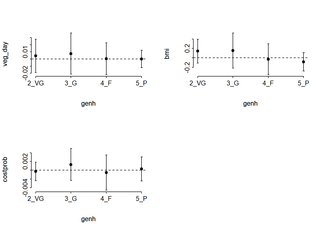
par(mfrow= c(1,1))

From this plot, bmi (especially) and costprob vary as we move from the Very Good toward the Poor cutpoints, relative to veg_day, which is more stable.

27.9.10 Plotting the Fitted Model

27.9.10.1 Nomogram

fun.ge3 <- function(x) plogis(x - m2_lrm$coef[1] + m2_lrm$coef[2])
fun.ge4 <- function(x) plogis(x - m2_lrm$coef[1] + m2_lrm$coef[3])
fun.ge5 <- function(x) plogis(x - m2_lrm$coef[1] + m2_lrm$coef[4])

plot(nomogram(m2_lrm, fun=list('Prob Y >= 2 (VG or worse)' = plogis, 
                               'Prob Y >= 3 (Good or worse)' = fun.ge3,
                               'Prob Y >= 4 (Fair or Poor)' = fun.ge4,
                               'Prob Y = 5 (Poor)' = fun.ge5)))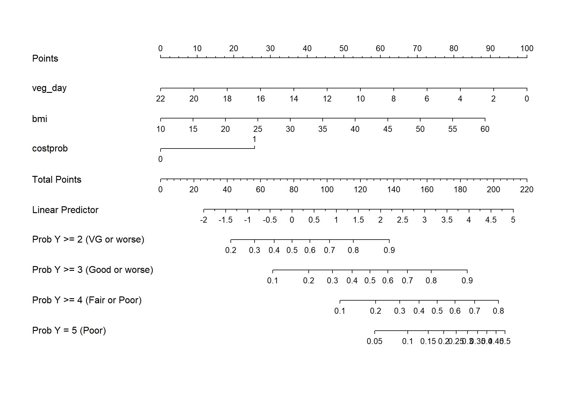

27.9.10.2 Using Predict and showing mean prediction on 1-5 scale

ggplot(Predict(m2_lrm, fun = Mean(m2_lrm, code = TRUE)))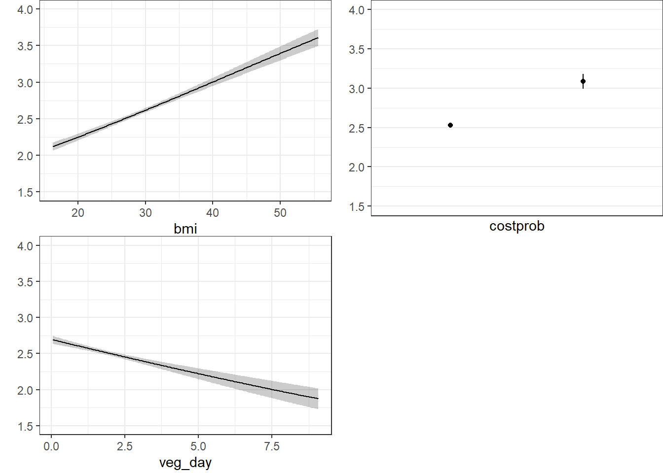

The nomogram and Predict results would be more interesting, of course, if we included a spline or interaction term. Let’s do that in model m3_lrm, and also add the incomegroup information.

27.10 A Larger Model, including income group

m3_lrm <- lrm(gen_n ~ rcs(veg_day,3) + rcs(bmi, 4) + 
                  incomegroup + catg(costprob) + 
                  bmi %ia% costprob, 
              data = sm1, x = T, y = T)

m3_lrm

Logistic Regression Model

lrm(formula = gen_n ~ rcs(veg_day, 3) + rcs(bmi, 4) + incomegroup + 
    catg(costprob) + bmi %ia% costprob, data = sm1, x = T, y = T)


Frequencies of Responses

   1    2    3    4    5 
 822 1805 1667  801  299 

                       Model Likelihood      Discrimination    Rank Discrim.    
                             Ratio Test             Indexes          Indexes    
Obs          5394    LR chi2    1190.35      R2       0.209    C       0.696    
max |deriv| 1e-11    d.f.            14    R2(14,5394)0.196    Dxy     0.391    
                     Pr(> chi2) <0.0001    R2(14,4995)0.210    gamma   0.392    
                                             Brier    0.214    tau-a   0.291    

                   Coef    S.E.   Wald Z Pr(>|Z|)
y>=2                3.7535 0.4852   7.74 <0.0001 
y>=3                1.8717 0.4838   3.87 0.0001  
y>=4                0.2035 0.4831   0.42 0.6737  
y>=5               -1.4386 0.4846  -2.97 0.0030  
veg_day            -0.2602 0.0633  -4.11 <0.0001 
veg_day'            0.1756 0.0693   2.53 0.0113  
bmi                -0.0325 0.0203  -1.60 0.1086  
bmi'                0.5422 0.0989   5.48 <0.0001 
bmi''              -1.4579 0.2663  -5.47 <0.0001 
incomegroup=10-14K  0.2445 0.1705   1.43 0.1516  
incomegroup=15-19K -0.2626 0.1582  -1.66 0.0969  
incomegroup=20-24K -0.6434 0.1501  -4.29 <0.0001 
incomegroup=25-34K -0.7427 0.1459  -5.09 <0.0001 
incomegroup=35-49K -1.1621 0.1415  -8.21 <0.0001 
incomegroup=50-74K -1.4579 0.1418 -10.28 <0.0001 
incomegroup=75K+   -1.8592 0.1361 -13.66 <0.0001 
costprob=1          1.4576 0.3528   4.13 <0.0001 
bmi * costprob     -0.0259 0.0116  -2.24 0.0250

Another option here would have been to consider building incomegroup as a scored variable, with an order on its own, but I won’t force that here. Here’s the polr version…

m3 <- polr(genh ~ rcs(veg_day,3) + rcs(bmi, 4) + 
               incomegroup + costprob + 
               bmi %ia% costprob, data = sm1)

27.10.1 Cross-Tabulation of Predicted/Observed Classifications

addmargins(table(predict(m3), sm1$genh))

      
        1-E 2_VG  3_G  4_F  5_P  Sum
  1-E     3    2    0    0    0    5
  2_VG  642 1200  815  221   49 2927
  3_G   170  565  754  468  182 2139
  4_F     7   37   96  108   65  313
  5_P     0    1    2    4    3   10
  Sum   822 1805 1667  801  299 5394

This model predicts more Fair results, but still far too many Very Good with no Excellent at all.

27.10.2 Nomogram

fun.ge3 <- function(x) plogis(x - m3_lrm$coef[1] + m3_lrm$coef[2])
fun.ge4 <- function(x) plogis(x - m3_lrm$coef[1] + m3_lrm$coef[3])
fun.ge5 <- function(x) plogis(x - m3_lrm$coef[1] + m3_lrm$coef[4])

plot(nomogram(m3_lrm, fun=list('Prob Y >= 2 (VG or worse)' = plogis, 
                               'Prob Y >= 3 (Good or worse)' = fun.ge3,
                               'Prob Y >= 4 (Fair or Poor)' = fun.ge4,
                               'Prob Y = 5 (Poor)' = fun.ge5)))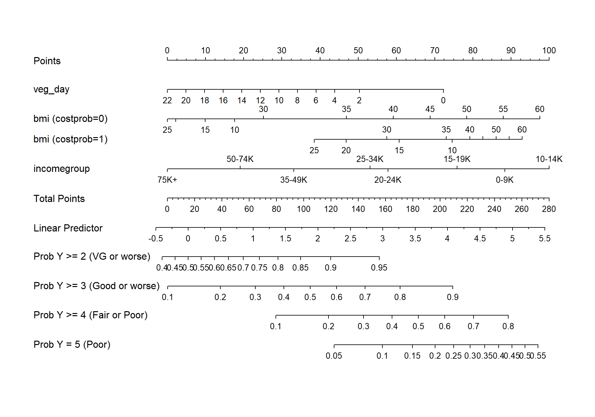

27.10.3 Using Predict and showing mean prediction on 1-5 scale

ggplot(Predict(m3_lrm, fun = Mean(m3_lrm, code = TRUE)))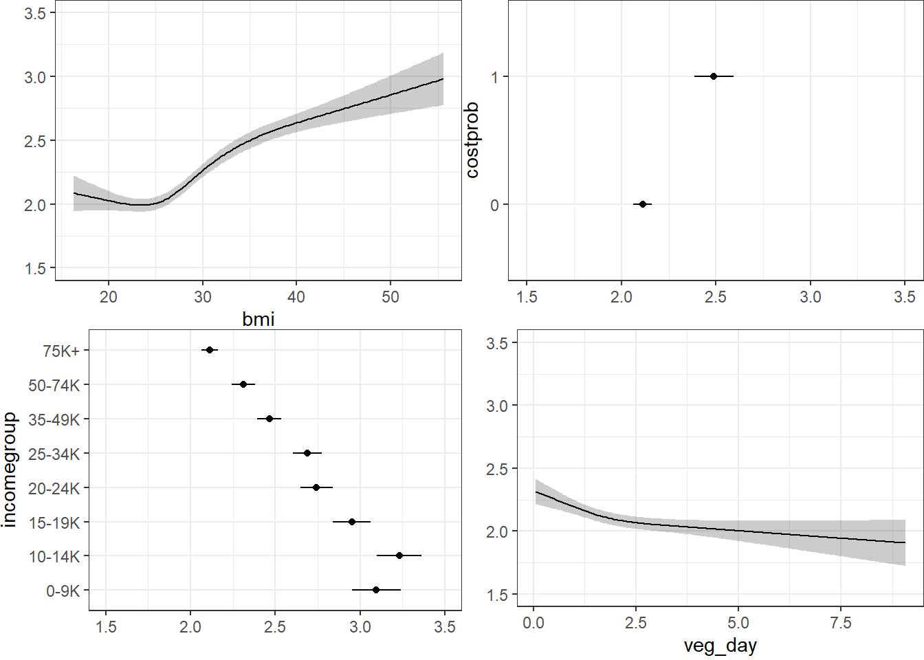

Here, we’re plotting the mean score on the 1-5 gen_n scale.

27.10.4 Validating the Summary Statistics in `m3_lrm`

set.seed(43221); validate(m3_lrm)

          index.orig training    test optimism index.corrected  n
Dxy           0.3915   0.3928  0.3899   0.0029          0.3886 40
R2            0.2093   0.2112  0.2071   0.0041          0.2053 40
Intercept     0.0000   0.0000  0.0019  -0.0019          0.0019 40
Slope         1.0000   1.0000  0.9871   0.0129          0.9871 40
Emax          0.0000   0.0000  0.0032   0.0032          0.0032 40
D             0.2205   0.2227  0.2179   0.0049          0.2156 40
U            -0.0004  -0.0004 -1.4667   1.4663         -1.4667 40
Q             0.2209   0.2231  1.6845  -1.4614          1.6823 40
B             0.2137   0.2134  0.2142  -0.0007          0.2145 40
g             1.0363   1.0410  1.0276   0.0133          1.0229 40
gp            0.2262   0.2265  0.2244   0.0022          0.2240 40

Still not very impressive, but much better than where we started. It’s not crazy to suggest that in new data, we might expect a Nagelkerke \(R^2\) of 0.205 and a C statistic of 0.5 + (0.3886/2) = 0.6943.

27.11 References for this Chapter

Some of the material here is adapted from http://stats.idre.ucla.edu/r/dae/ordinal-logistic-regression/.
I also found great guidance at http://data.library.virginia.edu/fitting-and-interpreting-a-proportional-odds-model/
Other parts are based on the work of Jeffrey S. Simonoff (2003) Analyzing Categorical Data in Chapter 10. Related data and R code are available at http://people.stern.nyu.edu/jsimonof/AnalCatData/Splus/.
Another good source for a simple example is https://onlinecourses.science.psu.edu/stat504/node/177.
Also helpful is https://onlinecourses.science.psu.edu/stat504/node/178 which shows a more complex example nicely.