24  Modeling a Count Outcome

In this chapter, and the next two chapters, I use a count outcome (# of poor physical health days out of the last 30) in OHIO SMART data created in Chapter 6 to demonstrate regression models for count outcomes.

Methods discussed in the chapter include:

• Ordinary Least Squares
• Poisson Regression
• Overdispersed Quasi-Poisson Regression

24.1 R Setup Used Here

knitr::opts_chunk$set(comment = NA)

library(broom)
library(boot)
library(countreg)
library(topmodels)
library(GGally)
library(lmtest)
library(rms)
library(sandwich)
library(tidyverse) 

theme_set(theme_bw())

24.2 Data Load

smart_oh <- readRDS("data/smart_ohio.Rds")

24.3 Creating A Useful Analytic Subset, ohioA

For this work, I’ll include the subset of all observations in smart_oh with complete data on these 14 variables.

Variable	Description
SEQNO	Subject identification code
mmsa_name	Name of statistical area
genhealth	Five categories (E, VG, G, F, P) on general health
physhealth	Now thinking about your physical health, which includes physical illness and injury, for how many days during the past 30 days was your physical health not good?
menthlth	Now thinking about your mental health, which includes stress, depression, and problems with emotions, for how many days during the past 30 days was your mental health not good?
healthplan	1 if the subject has any kind of health care coverage, 0 otherwise
costprob	1 indicates Yes to “Was there a time in the past 12 months when you needed to see a doctor but could not because of cost?”
agegroup	13 age groups from 18 through 80+
female	1 if subject is female
incomegroup	8 income groups from < 10,000 to 75,000 or more
bmi	body-mass index
smoke100	1 if Yes to “Have you smoked at least 100 cigarettes in your entire life?”
alcdays	# of days out of the past 30 on which the subject had at least one alcoholic drink

ohioA <- smart_oh |>
    select(SEQNO, mmsa_name, genhealth, physhealth, 
           menthealth, healthplan, costprob, 
           agegroup, female, incomegroup, bmi, smoke100, 
           alcdays) |>
    drop_na()

24.3.1 Is age group associated with physhealth?

ggplot(ohioA, aes(x = agegroup, y = physhealth)) +
    geom_violin(col = "blue")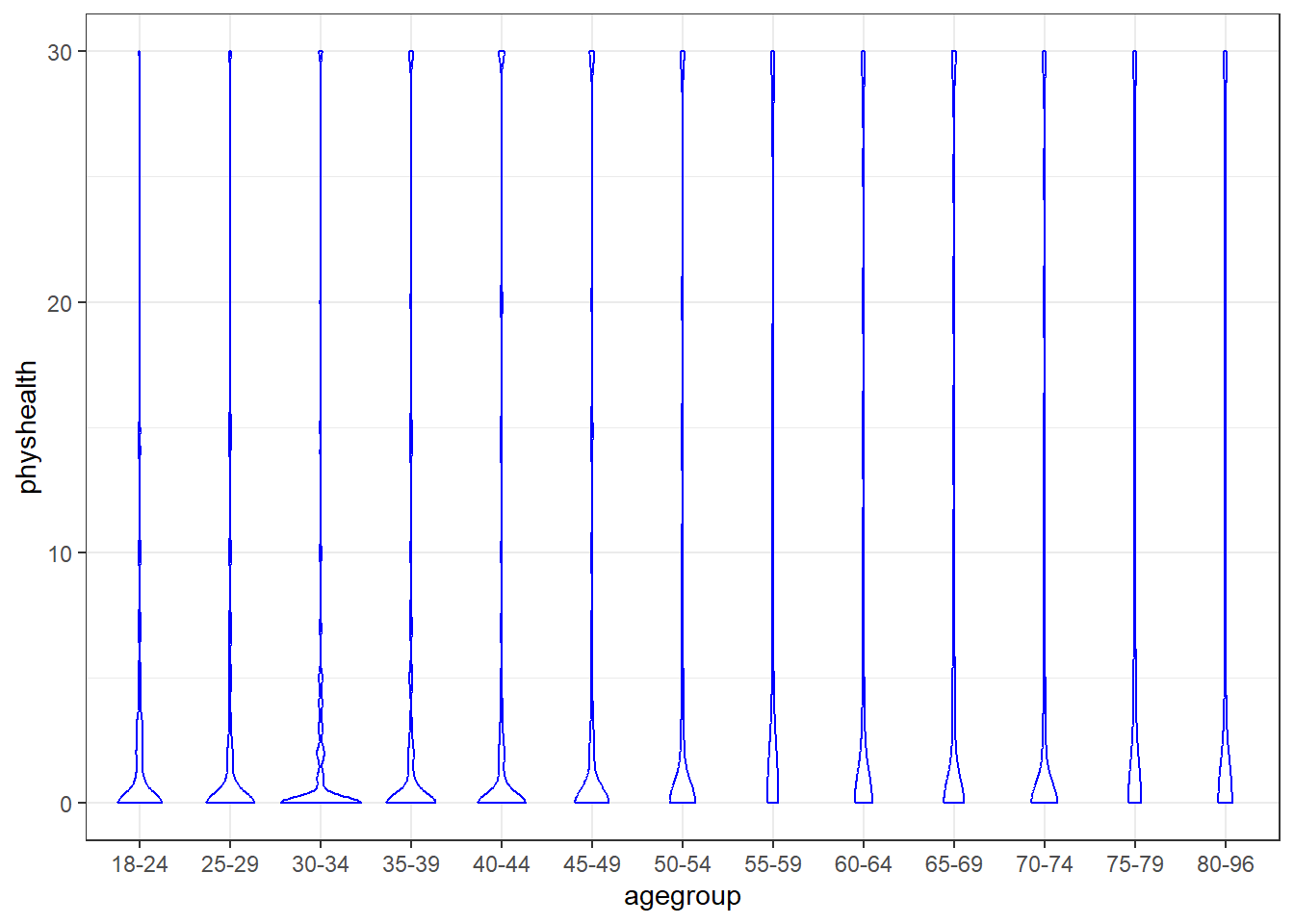

It’s hard to see much of anything here. The main conclusion seems to be that 0 is by far the most common response.

Here’s a table by age group of:

• the number of respondents in that age group,
• the group’s mean physhealth response (remember that these are the number of poor physical health days in the last 30),
• their median physhealth response (which turns out to be 0 in each group), and
• the percentage of group members who responded 0.

ohioA |> group_by(agegroup) |>
    summarize(n = n(), mean = round(mean(physhealth),2), 
              median = median(physhealth),
              percent_0s = round(100*sum(physhealth == 0)/n,1))

# A tibble: 13 × 5
   agegroup     n  mean median percent_0s
   <fct>    <int> <dbl>  <dbl>      <dbl>
 1 18-24      297  2.31      0       59.6
 2 25-29      259  2.53      0       66  
 3 30-34      296  2.14      0       69.3
 4 35-39      366  3.67      0       63.9
 5 40-44      347  4.18      0       62.8
 6 45-49      409  4.46      0       63.3
 7 50-54      472  4.76      0       60.4
 8 55-59      608  6.71      0       57.1
 9 60-64      648  5.9       0       57.6
10 65-69      604  6.09      0       56  
11 70-74      490  4.89      0       61.6
12 75-79      338  6.38      0       54.1
13 80-96      374  6.1       0       56.4

We can see a real change between the 45-49 age group and the 50-54 age group. The mean difference is clear from the table above, and the plot below (of the percentage with a zero response) in each age group identifies the same story.

ohioA |> group_by(agegroup) |>
    summarize(n = n(), 
              percent_0s = round(100*sum(physhealth == 0)/n,1)) |>
    ggplot(aes(y = agegroup, x = percent_0s)) +
    geom_label(aes(label = percent_0s)) +
    labs(x = "% with no Bad Physical Health Days in last 30",
         y = "Age Group")

It looks like we have a fairly consistent result in the younger age range (18-49) or the older range (50+). On the theory that most of the people reading this document are in that younger range, we’ll focus on those respondents in what follows.

24.4 Exploratory Data Analysis (in the 18-49 group)

We want to predict the 0-30 physhealth count variable for the 18-49 year old respondents.

To start, we’ll use two predictors:

• the respondent’s body mass index, and
• whether the respondent has smoked 100 cigarettes in their lifetime.

We anticipate that each of these variables will have positive associations with the physhealth score. That is, heavier people, and those who have used tobacco will be less healthy, and thus have higher numbers of poor physical health days.

24.4.1 Build a subset of those ages 18-49

First, we’ll identify the subset of respondents who are between 18 and 49 years of age.

ohioA_young.raw <- ohioA |>
    filter(agegroup %in% c("18-24", "25-29", "30-34", 
                           "35-39", "40-44", "45-49")) |>
    droplevels()

ohioA_young.raw |> 
    select(physhealth, bmi, smoke100, agegroup) |>
    summary()

   physhealth          bmi           smoke100       agegroup  
 Min.   : 0.000   Min.   :14.00   Min.   :0.0000   18-24:297  
 1st Qu.: 0.000   1st Qu.:23.74   1st Qu.:0.0000   25-29:259  
 Median : 0.000   Median :27.32   Median :0.0000   30-34:296  
 Mean   : 3.337   Mean   :28.79   Mean   :0.4189   35-39:366  
 3rd Qu.: 2.000   3rd Qu.:32.43   3rd Qu.:1.0000   40-44:347  
 Max.   :30.000   Max.   :75.52   Max.   :1.0000   45-49:409  

24.4.2 Centering bmi

I’m going to center the bmi variable to help me interpret the final models later.

ohioA_young <- ohioA_young.raw |>
    mutate(bmi_c = bmi - mean(bmi)) 

Now, let’s look more closely at the distribution of these variables, starting with our outcome.

24.4.3 Distribution of the Outcome

What’s the distribution of physhealth?

ggplot(ohioA_young.raw, aes(x = physhealth)) +
    geom_histogram(binwidth = 1, fill = "red", col = "white")

ohioA_young.raw |>
    count(physhealth == 0, physhealth == 30)

# A tibble: 3 × 3
  `physhealth == 0` `physhealth == 30`     n
  <lgl>             <lgl>              <int>
1 FALSE             FALSE                612
2 FALSE             TRUE                  98
3 TRUE              FALSE               1264

Most of our respondents said zero, the minimum allowable value, although there is also a much smaller bump at 30, the maximum value we will allow.

Dealing with this distribution is going to be a bit of a challenge. We will develop a series of potential modeling approaches for this sort of data, but before we do that, let’s look at the distribution of our other two variables, and the pairwise associations, in a scatterplot matrix.

24.4.4 Scatterplot Matrix

Now, here’s the scatterplot matrix for those 1974 subjects, using the centered bmi data captured in the bmi_c variable.

temp <- ohioA_young |> select(bmi_c, smoke100, physhealth)

ggpairs(temp)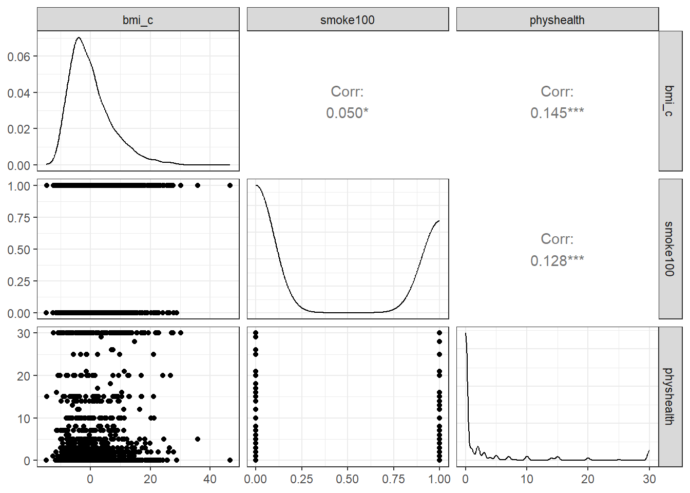

So bmi_c and smoke100 each have modest positive correlations with physhealth and only a very small correlation with each other. Here are some summary statistics for this final data.

24.4.5 Summary of the final subset of data

Remember that since the mean of bmi is 28.8, the bmi_c values are just bmi - 28.8 for each subject.

ohioA_young |> 
    select(bmi, bmi_c, smoke100, physhealth) |>
    summary()

      bmi            bmi_c            smoke100        physhealth    
 Min.   :14.00   Min.   :-14.791   Min.   :0.0000   Min.   : 0.000  
 1st Qu.:23.74   1st Qu.: -5.051   1st Qu.:0.0000   1st Qu.: 0.000  
 Median :27.32   Median : -1.471   Median :0.0000   Median : 0.000  
 Mean   :28.79   Mean   :  0.000   Mean   :0.4189   Mean   : 3.337  
 3rd Qu.:32.43   3rd Qu.:  3.636   3rd Qu.:1.0000   3rd Qu.: 2.000  
 Max.   :75.52   Max.   : 46.729   Max.   :1.0000   Max.   :30.000  

24.5 Modeling Strategies Explored Here

We are going to predict physhealth using bmi_c and smoke100.

• Remember that physhealth is a count of the number of poor physical health days in the past 30.
• As a result, physhealth is restricted to taking values between 0 and 30.

We will demonstrate the use of each of the following regression models, some of which are better choices than others.

1. Ordinary Least Squares (OLS) predicting physhealth
2. OLS predicting the logarithm of (physhealth + 1)
3. Poisson regression, which is appropriate for predicting counts
4. Poisson regression, adjusted to account for overdispersion

and, in Chapter 25:

5. Negative binomial regression, also used for counts and which adjusts for overdispersion

and, in Chapter 26:

6. Zero-inflated models, in both the Poisson and Negative Binomial varieties, which allow us to fit counts that have lots of zero values
7. A “hurdle” model, which allows us to separately fit a model to predict the incidence of “0” and then a separate model to predict the value of physhealth when we know it is not zero
8. Tobit regression, where a lower (and upper) bound may be set, but the underlying model describes a latent variable which can extend beyond these boundaries

24.5.1 What Will We Demonstrate?

With each approach, we will fit the model and specify procedures for doing so in R. Then we will:

1. Specify the fitted model equation
2. Interpret the model’s coefficient estimates and 95% confidence intervals around those estimates.
3. Perform a test of whether each variable adds value to the model, when the other one is already included.
4. Store the fitted values and appropriate residuals for each model.
5. Summarize the model’s apparent \(R^2\) value, the proportion of variation explained, and the model log likelihood.
6. Perform checks of model assumptions as appropriate.
7. Describe how predictions would be made for two new subjects.
   • Harry has a BMI that is 10 kg/m² higher than the average across all respondents and has smoked more than 100 cigarettes in his life.
   • Sally has a BMI that is 5 kg/m² less than the average across all respondents and has not smoked more than 100 cigarettes in her life.

In addition, for some of the new models, we provide a little of the mathematical background, and point to other resources you can use to learn more about the model.

24.5.2 Extra Data File for Harry and Sally

To make our lives a little easier, I’ll create a little tibble containing the necessary data for Harry and Sally.

hs_data <- tibble(subj = c("Harry", "Sally"), 
                  bmi_c = c(10, -5), smoke100 = c(1, 0))
hs_data

# A tibble: 2 × 3
  subj  bmi_c smoke100
  <chr> <dbl>    <dbl>
1 Harry    10        1
2 Sally    -5        0

24.6 The OLS Approach

mod_ols1 <- lm(physhealth ~ bmi_c + smoke100, 
               data = ohioA_young)

summary(mod_ols1)

Call:
lm(formula = physhealth ~ bmi_c + smoke100, data = ohioA_young)

Residuals:
     Min       1Q   Median       3Q      Max 
-11.1472  -3.6639  -2.2426  -0.7807  28.8777 

Coefficients:
            Estimate Std. Error t value Pr(>|t|)    
(Intercept)  2.57046    0.21648  11.874  < 2e-16 ***
bmi_c        0.14437    0.02305   6.263 4.61e-10 ***
smoke100     1.83061    0.33469   5.470 5.09e-08 ***
---
Signif. codes:  0 '***' 0.001 '**' 0.01 '*' 0.05 '.' 0.1 ' ' 1

Residual standard error: 7.328 on 1971 degrees of freedom
Multiple R-squared:  0.0356,    Adjusted R-squared:  0.03462 
F-statistic: 36.37 on 2 and 1971 DF,  p-value: 3.072e-16

confint(mod_ols1)

                2.5 %   97.5 %
(Intercept) 2.1459143 2.995005
bmi_c       0.0991636 0.189573
smoke100    1.1742213 2.486995

24.6.1 Interpreting the Coefficients

• The intercept, 2.57, is the predicted physhealth (in days) for a subject with average BMI who has not smoked 100 cigarettes or more.
• The bmi_c coefficient, 0.144, indicates that for each additional kg/m² of BMI, while holding smoke100 constant, the predicted physhealth value increases by 0.144 day.
• The smoke100 coefficient, 1.83, indicates that a subject who has smoked 100 cigarettes or more has a predicted physhealth value 1.83 days larger than another subject with the same bmi but who has not smoked 100 cigarettes.

24.6.2 Store fitted values and residuals

We can use broom to do this. Here, for instance, is a table of the first six predictions and residuals.

sm_ols_1 <- augment(mod_ols1, ohioA_young)

sm_ols_1 |> select(physhealth, .fitted, .resid) |> head()

# A tibble: 6 × 3
  physhealth .fitted .resid
       <dbl>   <dbl>  <dbl>
1          0    2.13  -2.13
2          0    2.25  -2.25
3          0    3.14  -3.14
4         30    5.72  24.3 
5          0    3.20  -3.20
6          0    3.83  -3.83

It turns out that 0 of the 1974 predictions that we make are below 0, and the largest prediction made by this model is 11.15 days.

24.6.3 Specify the \(R^2\) and log(likelihood) values

The glance function in the broom package gives us the raw and adjusted \(R^2\) values, and the model log(likelihood), among other summaries.

glance(mod_ols1) |> round(3)

# A tibble: 1 × 12
  r.squared adj.r.squared sigma statistic p.value    df logLik    AIC    BIC
      <dbl>         <dbl> <dbl>     <dbl>   <dbl> <dbl>  <dbl>  <dbl>  <dbl>
1     0.036         0.035  7.33      36.4       0     2 -6731. 13470. 13492.
# ℹ 3 more variables: deviance <dbl>, df.residual <dbl>, nobs <dbl>

Here, we have

Model	\(R^2\)	log(likelihood)
OLS	0.036	-6730.98

24.6.4 Check model assumptions

Here is a plot of the residuals vs. the fitted values for this OLS model.

ggplot(sm_ols_1, aes(x = .fitted, y = .resid)) +
    geom_point() +
    labs(title = "Residuals vs. Fitted Values for OLS model")

As usual, we can check OLS assumptions (linearity, homoscedasticity and normality) with R’s complete set of residual plots.

par(mfrow = c(2,2))
plot(mod_ols1)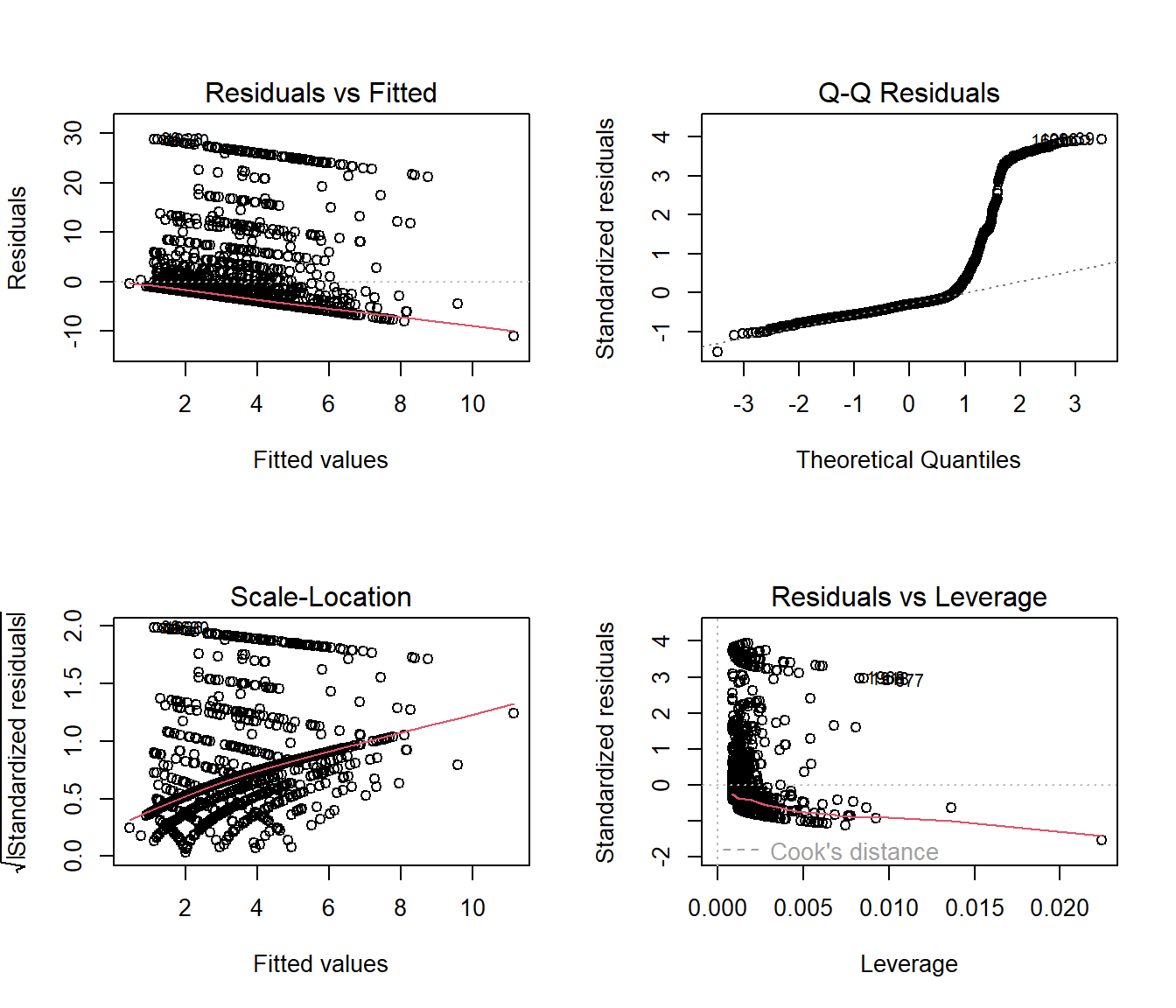

par(mfrow = c(1,1))

We see the problem with our residuals. They don’t follow a Normal distribution.

24.6.5 Predictions for Harry and Sally

predict(mod_ols1, newdata = hs_data,
        interval = "prediction")

       fit        lwr      upr
1 5.844750  -8.541164 20.23067
2 1.848618 -12.529923 16.22716

The prediction for Harry is 5.8 days, and for Sally is 1.8 days. The prediction intervals for each include some values below 0, even though 0 is the smallest possible value.

24.6.6 Notes

• This model could have been estimated using the ols function in the rms package, as well.

dd <- datadist(ohioA_young)
options(datadist = "dd")

(mod_ols1a <- ols(physhealth ~ bmi_c + smoke100,
                 data = ohioA_young, x = TRUE, y = TRUE))

Linear Regression Model

ols(formula = physhealth ~ bmi_c + smoke100, data = ohioA_young, 
    x = TRUE, y = TRUE)

                Model Likelihood    Discrimination    
                      Ratio Test           Indexes    
Obs    1974    LR chi2     71.55    R2       0.036    
sigma7.3276    d.f.            2    R2 adj   0.035    
d.f.   1971    Pr(> chi2) 0.0000    g        1.570    

Residuals

     Min       1Q   Median       3Q      Max 
-11.1472  -3.6639  -2.2426  -0.7807  28.8777 

          Coef   S.E.   t     Pr(>|t|)
Intercept 2.5705 0.2165 11.87 <0.0001 
bmi_c     0.1444 0.0230  6.26 <0.0001 
smoke100  1.8306 0.3347  5.47 <0.0001 

24.7 OLS model on log(physhealth + 1) days

We could try to solve the problem of fitting some predictions below 0 by log-transforming the data, so as to force values to be at least 0. Since we have undefined values when we take the log of 0, we’ll add one to each of the physhealth values before taking logs, and then transform back when we want to make predictions.

mod_ols_log1 <- lm(log(physhealth + 1) ~ bmi_c + smoke100,
                   data = ohioA_young)

summary(mod_ols_log1)

Call:
lm(formula = log(physhealth + 1) ~ bmi_c + smoke100, data = ohioA_young)

Residuals:
    Min      1Q  Median      3Q     Max 
-1.7079 -0.7058 -0.5051  0.5053  3.0484 

Coefficients:
            Estimate Std. Error t value Pr(>|t|)    
(Intercept)  0.57746    0.03099  18.634  < 2e-16 ***
bmi_c        0.01912    0.00330   5.796 7.91e-09 ***
smoke100     0.23679    0.04791   4.942 8.38e-07 ***
---
Signif. codes:  0 '***' 0.001 '**' 0.01 '*' 0.05 '.' 0.1 ' ' 1

Residual standard error: 1.049 on 1971 degrees of freedom
Multiple R-squared:  0.03003,   Adjusted R-squared:  0.02905 
F-statistic: 30.51 on 2 and 1971 DF,  p-value: 8.897e-14

confint(mod_ols_log1)

                 2.5 %     97.5 %
(Intercept) 0.51668682 0.63823590
bmi_c       0.01265192 0.02559421
smoke100    0.14282518 0.33075147

24.7.1 Interpreting the Coefficients

• The intercept, 0.58, is the predicted logarithm of (physhealth + 1) (in days) for a subject with average BMI who has not smoked 100 cigarettes or more.
  • We can exponentiate to see that the prediction for (physhealth + 1) here is exp(0.58) = 1.79 so the predicted physhealth for a subject with average BMI who has not smoked 100 cigarettes is 0.79 days.
• The bmi_c coefficient, 0.019, indicates that for each additional kg/m² of BMI, while holding smoke100 constant, the predicted logarithm of (physhealth + 1) increases by 0.019
• The smoke100 coefficient, 0.24, indicates that a subject who has smoked 100 cigarettes or more has a predicted log of (physhealth + 1) value that is 0.24 larger than another subject with the same bmi but who has not smoked 100 cigarettes.

24.7.2 Store fitted values and residuals

We can use broom to help us with this. Here, for instance, is a table of the first six predictions and residuals, on the scale of our transformed response, log(physhealth + 1).

sm_ols_log1 <- augment(mod_ols_log1, ohioA_young)

sm_ols_log1 <- sm_ols_log1 |> 
    mutate(outcome = log(physhealth + 1))

sm_ols_log1 |> 
    select(physhealth, outcome, .fitted, .resid) |>
    head()

# A tibble: 6 × 4
  physhealth outcome .fitted .resid
       <dbl>   <dbl>   <dbl>  <dbl>
1          0    0      0.520 -0.520
2          0    0      0.535 -0.535
3          0    0      0.647 -0.647
4         30    3.43   0.995  2.44 
5          0    0      0.656 -0.656
6          0    0      0.739 -0.739

Note that the outcome used in this model is log(physhealth + 1), so the .fitted and .resid values react to that outcome, and not to our original physhealth.

Another option would be to calculate the model-predicted physhealth, which I’ll call ph for a moment, with the formula:

\[ ph = e^{.fitted} - 1 \]

sm_ols_log1 <- sm_ols_log1 |> 
    mutate(pred.physhealth = exp(.fitted) - 1,
           res.physhealth = physhealth - pred.physhealth)

sm_ols_log1 |>
    select(physhealth, pred.physhealth, res.physhealth) |> 
    head()

# A tibble: 6 × 3
  physhealth pred.physhealth res.physhealth
       <dbl>           <dbl>          <dbl>
1          0           0.681         -0.681
2          0           0.708         -0.708
3          0           0.910         -0.910
4         30           1.70          28.3  
5          0           0.926         -0.926
6          0           1.09          -1.09 

It turns out that 0 of the 1974 predictions that we make are below 0, and the largest prediction made by this model is 4.52 days.

24.7.3 Specify the \(R^2\) and log(likelihood) values

The glance function in the broom package gives us the raw and adjusted \(R^2\) values, and the model log(likelihood), among other summaries.

glance(mod_ols_log1) |> round(3)

# A tibble: 1 × 12
  r.squared adj.r.squared sigma statistic p.value    df logLik   AIC   BIC
      <dbl>         <dbl> <dbl>     <dbl>   <dbl> <dbl>  <dbl> <dbl> <dbl>
1      0.03         0.029  1.05      30.5       0     2 -2894. 5796. 5818.
# ℹ 3 more variables: deviance <dbl>, df.residual <dbl>, nobs <dbl>

Here, we have

Model	Scale	\(R^2\)	log(likelihood)
OLS on log	log(physhealth + 1)	0.03	-2893.83

24.7.4 Getting \(R^2\) on the scale of physhealth

We could find the correlation of our model-predicted physhealth values, after back-transformation, and our observed physhealth values, if we wanted to, and then square that to get a sort of \(R^2\) value. But this model is not linear in physhealth, of course, so it’s not completely comparable to our prior OLS model.

24.7.5 Check model assumptions

As usual, we can check OLS assumptions (linearity, homoscedasticity and normality) with R’s complete set of residual plots. Of course, these residuals and fitted values are now on the log(physhealth + 1) scale.

par(mfrow = c(2,2))
plot(mod_ols_log1)

par(mfrow = c(1,1))

24.7.6 Predictions for Harry and Sally

predict(mod_ols_log1, newdata = hs_data, 
        interval = "prediction", type = "response")

       fit       lwr      upr
1 1.005480 -1.053893 3.064854
2 0.481846 -1.576472 2.540164

Again, these predictions are on the log(physhealth + 1) scale, and so we have to exponentiate them, and then subtract 1, to see them on the original physhealth scale.

exp(predict(mod_ols_log1, newdata = hs_data, 
            interval = "prediction", type = "response")) - 1

        fit        lwr      upr
1 1.7332198 -0.6514221 20.43133
2 0.6190605 -0.7932970 11.68175

The prediction for Harry is now 1.73 days, and for Sally is 0.62 days. The prediction intervals for each again include some values below 0, which is the smallest possible value.

24.8 A Poisson Regression Model

The physhealth data describe a count. Specifically a count of the number of days where the subject felt poorly in the last 30. Why wouldn’t we model this count with linear regression?

• A count can only be positive. Linear regression would estimate some subjects as having negative counts.
• A count is unlikely to follow a Normal distribution. In fact, it’s far more likely that the log of the counts will follow a Poisson distribution.

So, we’ll try that. The Poisson distribution is used to model a count outcome - that is, an outcome with possible values (0, 1, 2, …). The model takes a somewhat familiar form to the models we’ve used for linear and logistic regression¹. If our outcome is y and our linear predictors X, then the model is:

\[ y_i \sim \mbox{Poisson}(\lambda_i) \]

The parameter \(\lambda\) must be positive, so it makes sense to fit a linear regression on the logarithm of this…

\[ \lambda_i = exp(\beta_0 + \beta_1 X_1 + ... \beta_k X_k) \]

The coefficients \(\beta\) can be exponentiated and treated as multiplicative effects.

We’ll run a generalized linear model with a log link function, ensuring that all of the predicted values will be positive, and using a Poisson error distribution. This is called Poisson regression.

Poisson regression may be appropriate when the dependent variable is a count of events. The events must be independent - the occurrence of one event must not make any other more or less likely. That’s hard to justify in our case, but we can take a look.

mod_poiss1 <- glm(physhealth ~ bmi_c + smoke100, 
                  family = poisson(),
                  data = ohioA_young)

summary(mod_poiss1)

Call:
glm(formula = physhealth ~ bmi_c + smoke100, family = poisson(), 
    data = ohioA_young)

Coefficients:
            Estimate Std. Error z value Pr(>|z|)    
(Intercept) 0.906991   0.018699   48.51   <2e-16 ***
bmi_c       0.035051   0.001421   24.66   <2e-16 ***
smoke100    0.532505   0.024903   21.38   <2e-16 ***
---
Signif. codes:  0 '***' 0.001 '**' 0.01 '*' 0.05 '.' 0.1 ' ' 1

(Dispersion parameter for poisson family taken to be 1)

    Null deviance: 20222  on 1973  degrees of freedom
Residual deviance: 19151  on 1971  degrees of freedom
AIC: 21645

Number of Fisher Scoring iterations: 6

confint(mod_poiss1)

Waiting for profiling to be done...

                 2.5 %     97.5 %
(Intercept) 0.87011622 0.94342323
bmi_c       0.03225125 0.03782255
smoke100    0.48373882 0.58136497

24.8.1 The Fitted Equation

The model equation is

log(physhealth) = 0.91 + 0.035 bmi_c + 0.53 smoke100

It looks like both bmi and smoke_100 have confidence intervals excluding 0.

24.8.2 Interpreting the Coefficients

Our new model for \(y_i\) = counts of poor physhealth days in the last 30, follows the regression equation:

\[ y_i \sim \mbox{Poisson}(exp(0.91 + 0.035 bmi_c + 0.53 smoke100)) \]

where smoke100 is 1 if the subject has smoked 100 cigarettes (lifetime) and 0 otherwise, and bmi_c is just the centered body-mass index value in kg/m². We interpret the coefficients as follows:

• The constant term, 0.91, gives us the intercept of the regression - the prediction if smoke100 = 0 and bmi_c = 0. In this case, because we’ve centered BMI, it implies that exp(0.91) = 2.48 is the predicted days of poor physhealth for a non-smoker with average BMI.
• The coefficient of bmi_c, 0.035, is the expected difference in count of poor physhealth days (on the log scale) for each additional kg/m² of body mass index. The expected multiplicative increase is \(e^{0.035}\) = 1.036, corresponding to a 3.6% difference in the count.
• The coefficient of smoke100, 0.53, tells us that the predictive difference between those who have and who have not smoked 100 cigarettes can be found by multiplying the physhealth count by exp(0.53) = 1.7, yielding a 70% increase of the physhealth count.

As with linear or logistic regression, each coefficient is interpreted as a comparison where one predictor changes by one unit, while the others remain constant.

24.8.3 Testing the Predictors

We can use the Wald tests (z tests) provided with the Poisson regression output, or we can fit the model and then run an ANOVA to obtain a test based on the deviance (a simple transformation of the log likelihood ratio.)

• By the small p values in the Wald tests above, it seems that each predictor adds some predictive value to the model given the other predictor.
• The ANOVA approach for this model lets us check the impact of adding smoke100 to a model already containing bmi_c.

anova(mod_poiss1, test = "Chisq")

Analysis of Deviance Table

Model: poisson, link: log

Response: physhealth

Terms added sequentially (first to last)

         Df Deviance Resid. Df Resid. Dev  Pr(>Chi)    
NULL                      1973      20222              
bmi_c     1   609.46      1972      19612 < 2.2e-16 ***
smoke100  1   461.46      1971      19151 < 2.2e-16 ***
---
Signif. codes:  0 '***' 0.001 '**' 0.01 '*' 0.05 '.' 0.1 ' ' 1

To obtain a p value for smoke100’s impact after bmi_c is accounted for, we compare the difference in deviance to a chi-square distribution with 1 degree of freedom. To check the effect of bmi_c, we could refit the model with bmi_c entering last, and again run an ANOVA.

We could also run a likelihood-ratio test for each predictor, by fitting the model with and without that predictor.

mod_poiss1_without_bmi <- glm(physhealth ~ smoke100,
                              family = poisson(),
                              data = ohioA_young)

anova(mod_poiss1, mod_poiss1_without_bmi, test = "Chisq")

Analysis of Deviance Table

Model 1: physhealth ~ bmi_c + smoke100
Model 2: physhealth ~ smoke100
  Resid. Df Resid. Dev Df Deviance  Pr(>Chi)    
1      1971      19151                          
2      1972      19692 -1  -540.98 < 2.2e-16 ***
---
Signif. codes:  0 '***' 0.001 '**' 0.01 '*' 0.05 '.' 0.1 ' ' 1

24.8.4 Correcting for Overdispersion with coeftest/coefci

The main assumption we’ll think about in a Poisson model is about overdispersion. We might deal with the overdispersion we see in this model by changing the nature of the tests we run within this model, using the coeftest or coefci approaches from the lmtest package, as I’ll demonstrate next, or we might refit the model using a quasi-likelihood approach, as I’ll show in the material to come.

Here, we’ll use the coeftest and coefci approach from lmtest combined with robust sandwich estimation (via the sandwich package) to re-compute the Wald tests.

coeftest(mod_poiss1, vcov. = sandwich)

z test of coefficients:

             Estimate Std. Error z value  Pr(>|z|)    
(Intercept) 0.9069908  0.0717221 12.6459 < 2.2e-16 ***
bmi_c       0.0350508  0.0061178  5.7293 1.008e-08 ***
smoke100    0.5325053  0.1004300  5.3023 1.144e-07 ***
---
Signif. codes:  0 '***' 0.001 '**' 0.01 '*' 0.05 '.' 0.1 ' ' 1

coefci(mod_poiss1, vcov. = sandwich)

                 2.5 %     97.5 %
(Intercept) 0.76641801 1.04756366
bmi_c       0.02306016 0.04704145
smoke100    0.33566606 0.72934460

Both predictors still display small p values, but the standard errors are more appropriate. Later, we’ll fit this approach by changing the estimation method to a quasi-likelihood approach.

24.8.5 Store fitted values and residuals

What happens if we try using the broom package in this case? We can, if we like, get our residuals and predicted values right on the scale of our physhealth response.

sm_poiss1 <- augment(mod_poiss1, ohioA_young,
                     type.predict = "response")

sm_poiss1 |> 
    select(physhealth, .fitted) |>
    head()

# A tibble: 6 × 2
  physhealth .fitted
       <dbl>   <dbl>
1          0    2.23
2          0    2.29
3          0    3.10
4         30    5.32
5          0    3.15
6          0    3.68

24.8.6 Rootogram: see the fit of a count regression model

A rootogram is a very useful way to visualize the fit of a count regression model². The rootogram function in the topmodels package makes this pretty straightforward. By default, this fits a hanging rootogram on the square root of the frequencies.

rootogram(mod_poiss1, max = 30)

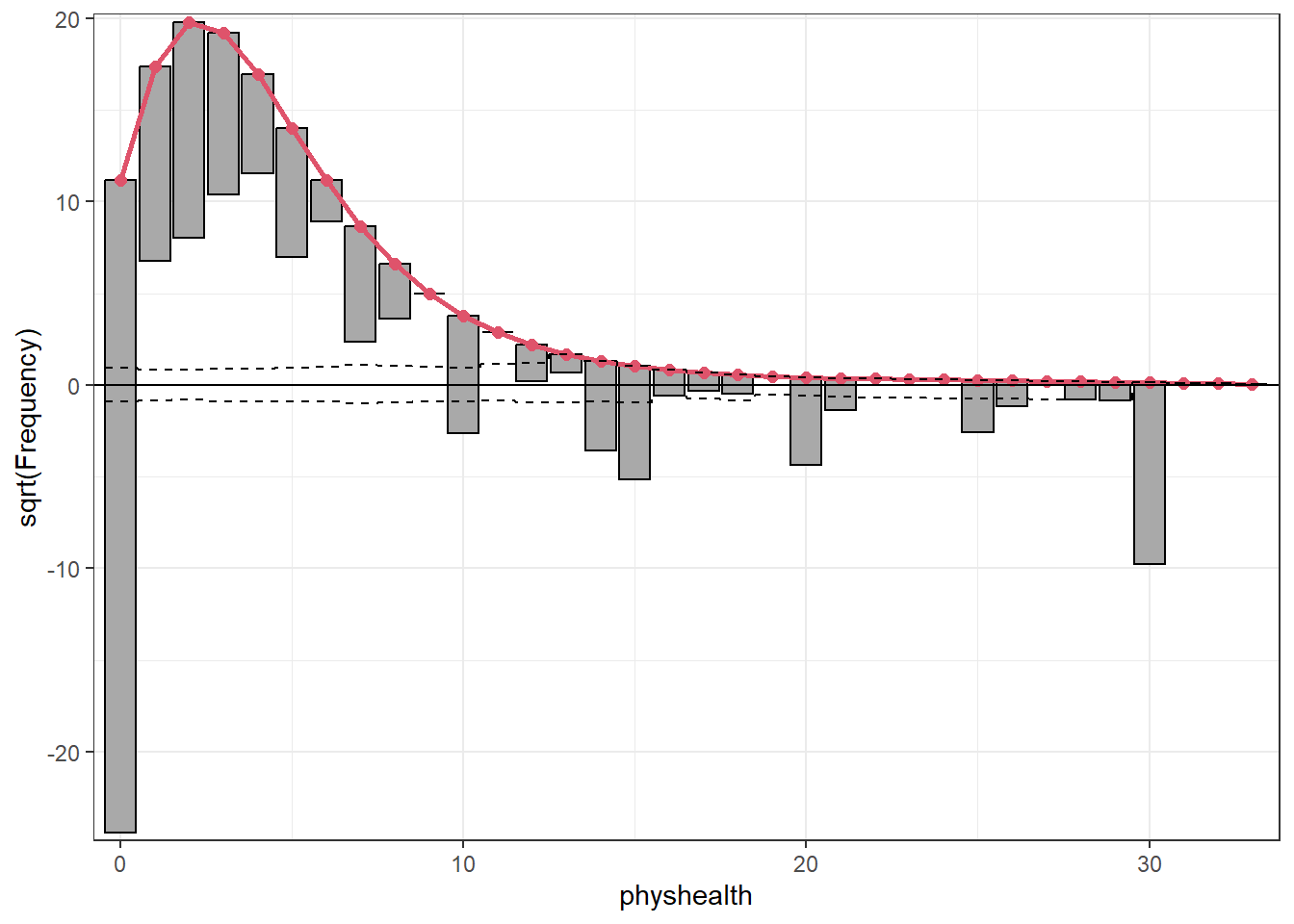
The red curved line is the theoretical Poisson fit. “Hanging” from each point on the red line is a bar, the height of which represents the difference between expected and observed counts. A bar hanging below 0 indicates underfitting. A bar hanging above 0 indicates overfitting. The counts have been transformed with a square root transformation to prevent smaller counts from getting obscured and overwhelmed by larger counts. We see a great deal of underfitting for counts of 0, and overfitting for most other counts, especially 1-6, with some underfitting again by physhealth above 14 days.

24.8.7 Specify the \(R^2\) and log(likelihood) values

We can calculate the \(R^2\) as the squared correlation of the fitted values and the observed values.

# The correlation of observed and fitted values
(poiss_r <- with(sm_poiss1, cor(physhealth, .fitted)))

[1] 0.1846814

# R-square
poiss_r^2

[1] 0.03410723

The glance function in the broom package gives us model log(likelihood), among other summaries.

glance(mod_poiss1) |> round(3)

# A tibble: 1 × 8
  null.deviance df.null  logLik    AIC    BIC deviance df.residual  nobs
          <dbl>   <dbl>   <dbl>  <dbl>  <dbl>    <dbl>       <dbl> <dbl>
1        20222.    1973 -10820. 21645. 21662.   19151.        1971  1974

Here, we have

Model	Scale	\(R^2\)	log(likelihood)
Poisson	log(physhealth)	0.034	-10189.33

24.8.8 Check model assumptions

The Poisson model is a classical generalized linear model, estimated using the method of maximum likelihood. While the default plot option for a glm still shows the plots we would use to assess the assumptions of an OLS model, we don’t actually get much from that, since our Poisson model has different assumptions. It can be useful to look at a plot of residuals vs. fitted values on the original physhealth scale.

ggplot(sm_poiss1, aes(x = .fitted, y = .resid)) +
    geom_point() +
    labs(title = "Residuals vs. Fitted `physhealth`",
         subtitle = "Original Poisson Regression model")

24.8.9 Using glm.diag.plots from the boot package

The glm.diag.plots function from the boot package makes a series of diagnostic plots for generalized linear models.

• (Top, Left) Jackknife deviance residuals against fitted values. This is essentially identical to what you obtain with plot(mod_poiss1, which = 1). A jackknife deviance residual is also called a likelihood residual. It is the change in deviance when this observation is omitted from the data.
• (Top, Right) Normal Q-Q plot of standardized deviance residuals. (Dotted line shows expectation if those standardized residuals followed a Normal distribution, and these residuals generally should.) The result is similar to what you obtain with plot(mod_poiss1, which = 2).
• (Bottom, Left) Cook statistic vs. standardized leverage
  • n = # of observations, p = # of parameters estimated
  • Horizontal dotted line is at \(\frac{8}{n - 2p}\). Points above the line have high influence on the model.
  • Vertical line is at \(\frac{2p}{n - 2p}\). Points to the right of the line have high leverage.
• (Bottom, Right) Index plot of Cook’s statistic to help identify the observations with high influence. This is essentially the same plot as plot(mod_poiss1, which = 4)

glm.diag.plots(mod_poiss1)

When working with these plots, it is possible to use the iden command to perform some interactive identification of points in your R terminal. But that doesn’t play out effectively in an HTML summary document like this, so we’ll leave that out.

24.8.10 Predictions for Harry and Sally

The predictions from a glm fit like this don’t include prediction intervals. But we can get predictions on the scale of our original response variable, physhealth, like this.

predict(mod_poiss1, newdata = hs_data, se.fit = TRUE,
        type = "response")

$fit
       1        2 
5.989478 2.078688 

$se.fit
         1          2 
0.11544326 0.04314273 

$residual.scale
[1] 1

By using response as the type, these predictions fall on the original physhealth scale. The prediction for Harry is now 5.99 days, and for Sally is 2.08 days.

24.9 Overdispersion in a Poisson Model

Poisson regressions do not supply an independent variance parameter \(\sigma\), and as a result can be overdispersed, and usually are. Under the Poisson distribution, the variance equals the mean - so the standard deviation equals the square root of the mean. The notion of overdispersion arises here. When fitting generalized linear models with Poisson error distributions, the residual deviance and its degrees of freedom should be approximately equal if the model fits well.

If the residual deviance is far greater than the degrees of freedom, then overdispersion may well be a problem. In this case, the residual deviance is about 8.5 times the size of the residual degrees of freedom, so that’s a clear indication of overdispersion. We saw earlier that the Poisson regression model requires that the outcome (here the physhealth counts) be independent. A possible reason for the overdispersion we see here is that physhealth on different days likely do not occur independently of one another but likely “cluster” together.

24.9.1 Testing for Overdispersion?

Gelman and Hill provide an overdispersion test in R for a Poisson model as follows…

yhat <- predict(mod_poiss1, type = "response")
n <- arm::display(mod_poiss1)$n

glm(formula = physhealth ~ bmi_c + smoke100, family = poisson(), 
    data = ohioA_young)
            coef.est coef.se
(Intercept) 0.91     0.02   
bmi_c       0.04     0.00   
smoke100    0.53     0.02   
---
  n = 1974, k = 3
  residual deviance = 19150.9, null deviance = 20221.8 (difference = 1070.9)

k <- arm::display(mod_poiss1)$k

glm(formula = physhealth ~ bmi_c + smoke100, family = poisson(), 
    data = ohioA_young)
            coef.est coef.se
(Intercept) 0.91     0.02   
bmi_c       0.04     0.00   
smoke100    0.53     0.02   
---
  n = 1974, k = 3
  residual deviance = 19150.9, null deviance = 20221.8 (difference = 1070.9)

z <- (ohioA_young$physhealth - yhat) / sqrt(yhat)
cat("overdispersion ratio is ", sum(z^2)/ (n - k), "\n")

overdispersion ratio is  15.58261 

cat("p value of overdispersion test is ", 
    pchisq(sum(z^2), df = n-k, lower.tail = FALSE), "\n")

p value of overdispersion test is  0 

The p value is very small, indicating that the probability is essentially zero that a random variable from a \(\chi^2\) distribution with (n - k) = 1971 degrees of freedom would be as large as what we observed in this case. So there is almost surely some overdispersion.

In summary, the physhealth counts are overdispersed by a factor of 15.581, which is enormous (even a factor of 2 would be considered large.) The basic correction for overdisperson is to multiply all regression standard errors by \(\sqrt{15.581}\) = 3.95.

The quasipoisson model and the negative binomial model that we’ll fit below are very similar. We write the overdispersed “quasiPoisson” model as:

\[ y_i \sim \mbox{overdispersed Poisson} (\mu_i exp(X_i \beta), \omega) \]

where \(\omega\) is the overdispersion parameter, 15.581, in our case. The Poisson model we saw previously is then just the overdispersed Poisson model with \(\omega = 1\).

24.10 Fitting the Quasi-Poisson Model

To deal with overdispersion, one useful approach is to apply a quasi-likelihood estimation procedure, as follows:

mod_poiss_od1 <- glm(physhealth ~ bmi_c + smoke100, 
                  family = quasipoisson(),
                  data = ohioA_young)

summary(mod_poiss_od1)

Call:
glm(formula = physhealth ~ bmi_c + smoke100, family = quasipoisson(), 
    data = ohioA_young)

Coefficients:
            Estimate Std. Error t value Pr(>|t|)    
(Intercept) 0.906991   0.073818  12.287  < 2e-16 ***
bmi_c       0.035051   0.005611   6.247 5.11e-10 ***
smoke100    0.532505   0.098308   5.417 6.81e-08 ***
---
Signif. codes:  0 '***' 0.001 '**' 0.01 '*' 0.05 '.' 0.1 ' ' 1

(Dispersion parameter for quasipoisson family taken to be 15.58436)

    Null deviance: 20222  on 1973  degrees of freedom
Residual deviance: 19151  on 1971  degrees of freedom
AIC: NA

Number of Fisher Scoring iterations: 6

confint(mod_poiss_od1)

Waiting for profiling to be done...

                 2.5 %     97.5 %
(Intercept) 0.75877174 1.04831740
bmi_c       0.02383574 0.04583252
smoke100    0.34039368 0.72606948

This “quasi-Poisson regression” model uses the same mean function as Poisson regression, but now estimated by quasi-maximum likelihood estimation or, equivalently, through the method of generalized estimating equations, where the inference is adjusted by an estimated dispersion parameter. Sometimes, though I won’t demonstrate this here, people fit an “adjusted” Poisson regression model, where this estimation by quasi-ML is augmented to adjust the inference via sandwich estimates of the covariances³.

24.10.1 The Fitted Equation

The model equation is still log(physhealth) = 0.91 + 0.035 bmi_c + 0.53 smoke100. The estimated coefficients still have small p values, but the standard errors for each coefficient are considerably larger when we account for overdispersion.

The dispersion parameter for the quasi-Poisson family is now taken to be a bit less than the square root of the ratio of the residual deviance and its degrees of freedom. This is a much more believable model, as a result.

24.10.2 Interpreting the Coefficients

No meaningful change from the Poisson model we saw previously.

24.10.3 Testing the Predictors

Again, we can use the Wald tests (z tests) provided with the Poisson regression output, or we can fit the model and then run an ANOVA to obtain a test based on the deviance (a simple transformation of the log likelihood ratio.)

• By the Wald tests shown above, each predictor appears to add some predictive value to the model given the other predictor.
• The ANOVA approach for this model lets us check the impact of adding smoke100 to a model already containing bmi_c.

anova(mod_poiss_od1, test = "Chisq")

Analysis of Deviance Table

Model: quasipoisson, link: log

Response: physhealth

Terms added sequentially (first to last)

         Df Deviance Resid. Df Resid. Dev  Pr(>Chi)    
NULL                      1973      20222              
bmi_c     1   609.46      1972      19612 4.011e-10 ***
smoke100  1   461.46      1971      19151 5.282e-08 ***
---
Signif. codes:  0 '***' 0.001 '**' 0.01 '*' 0.05 '.' 0.1 ' ' 1

The result is unchanged. To obtain a p value for smoke100’s impact after bmi_c is accounted for, we compare the difference in deviance to a chi-square distribution with 1 degree of freedom. The resulting p value is very small.

To check the effect of bmi_c, we could refit the model with and without bmi_c, and again run an ANOVA. I’ll skip that here.

24.10.4 Store fitted values and residuals

What happens if we try using the broom package in this case? We can, if we like, get our predicted values right on the scale of our physhealth response.

sm_poiss_od1 <- augment(mod_poiss_od1, ohioA_young,
                     type.predict = "response")

sm_poiss_od1 |> 
    select(physhealth, .fitted) |>
    head()

# A tibble: 6 × 2
  physhealth .fitted
       <dbl>   <dbl>
1          0    2.23
2          0    2.29
3          0    3.10
4         30    5.32
5          0    3.15
6          0    3.68

It turns out that 0 of the 1974 predictions that we make are below 0, and the largest prediction made by this model is 21.7 days.

The rootogram function we’ve shown doesn’t support overdispersed Poisson models at the moment.

24.10.5 Specify the \(R^2\) and log(likelihood) values

We can calculate the \(R^2\) as the squared correlation of the fitted values and the observed values.

# The correlation of observed and fitted values
(poiss_od_r <- with(sm_poiss_od1, cor(physhealth, .fitted)))

[1] 0.1846814

# R-square
poiss_od_r^2

[1] 0.03410723

The glance function in the broom package gives us model log(likelihood), among other summaries.

glance(mod_poiss_od1) |> round(3)

# A tibble: 1 × 8
  null.deviance df.null logLik   AIC   BIC deviance df.residual  nobs
          <dbl>   <dbl>  <dbl> <dbl> <dbl>    <dbl>       <dbl> <dbl>
1        20222.    1973     NA    NA    NA   19151.        1971  1974

Here, we have

Model	Scale	\(R^2\)	log(likelihood)
Poisson	log(physhealth)	0.034	NA

24.10.6 Check model assumptions

Having dealt with the overdispersion, this should be a cleaner model in some ways, but the diagnostics (other than the dispersion) will be the same. Here is a plot of residuals vs. fitted values on the original physhealth scale.

ggplot(sm_poiss_od1, aes(x = .fitted, y = .resid)) +
    geom_point() +
    labs(title = "Residuals vs. Fitted `physhealth`",
         subtitle = "Overdispersed Poisson Regression model")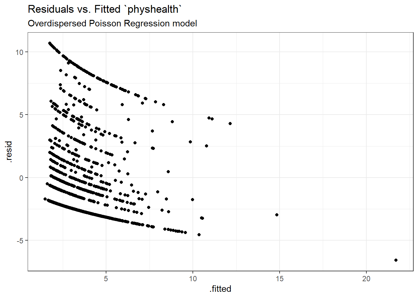

I’ll skip the glm.diag.plots results, since you’ve already seen them.

24.10.7 Predictions for Harry and Sally

The predictions from this overdispersed Poisson regression will match those in the original Poisson regression, but the standard error will be larger.

predict(mod_poiss_od1, newdata = hs_data, se.fit = TRUE,
        type = "response")

$fit
       1        2 
5.989478 2.078688 

$se.fit
        1         2 
0.4557357 0.1703147 

$residual.scale
[1] 3.947703

By using response as the type, these predictions fall on the original physhealth scale. Again, the prediction for Harry is 5.99 days, and for Sally is 2.08 days.

24.11 Poisson and Quasi-Poisson models using Glm from the rms package

The Glm function in the rms package can be used to fit both the original Poisson regression and the quasi-Poisson model accounting for overdispersion.

24.11.1 Refitting the original Poisson regression with Glm

d <- datadist(ohioA_young)
options(datadist = "d")

mod_poi_Glm_1 <- Glm(physhealth ~ bmi_c + smoke100,
                     family = poisson(), 
                     data = ohioA_young, 
                     x = T, y = T)

mod_poi_Glm_1

General Linear Model

Glm(formula = physhealth ~ bmi_c + smoke100, family = poisson(), 
    data = ohioA_young, x = T, y = T)

                       Model Likelihood    
                             Ratio Test    
          Obs1974    LR chi2    1070.93    
Residual d.f.1971    d.f.             2    
          g 0.418    Pr(> chi2) <0.0001    

          Coef   S.E.   Wald Z Pr(>|Z|)
Intercept 0.9070 0.0187 48.50  <0.0001 
bmi_c     0.0351 0.0014 24.66  <0.0001 
smoke100  0.5325 0.0249 21.38  <0.0001 

24.11.2 Refitting the overdispersed Poisson regression with Glm

d <- datadist(ohioA_young)
options(datadist = "d")

mod_poi_od_Glm_1 <- Glm(physhealth ~ bmi_c + smoke100,
                     family = quasipoisson(), 
                     data = ohioA_young, 
                     x = T, y = T)

mod_poi_od_Glm_1

General Linear Model

Glm(formula = physhealth ~ bmi_c + smoke100, family = quasipoisson(), 
    data = ohioA_young, x = T, y = T)

                       Model Likelihood    
                             Ratio Test    
          Obs1974    LR chi2    1070.93    
Residual d.f.1971    d.f.             2    
          g 0.418    Pr(> chi2) <0.0001    

          Coef   S.E.   Wald Z Pr(>|Z|)
Intercept 0.9070 0.0738 12.29  <0.0001 
bmi_c     0.0351 0.0056  6.25  <0.0001 
smoke100  0.5325 0.0983  5.42  <0.0001 

The big advantage here is that we have access to the usual ANOVA, summary, and nomogram features that rms brings to fitting models.

24.11.3 ANOVA on a Glm fit

anova(mod_poi_od_Glm_1)

                Wald Statistics          Response: physhealth 

 Factor     Chi-Square d.f. P     
 bmi_c      39.03      1    <.0001
 smoke100   29.34      1    <.0001
 TOTAL      74.39      2    <.0001

This shows the individual Wald \(\chi^2\) tests without having to refit the model.

24.11.4 ggplots from Glm fit

ggplot(Predict(mod_poi_od_Glm_1, fun = exp))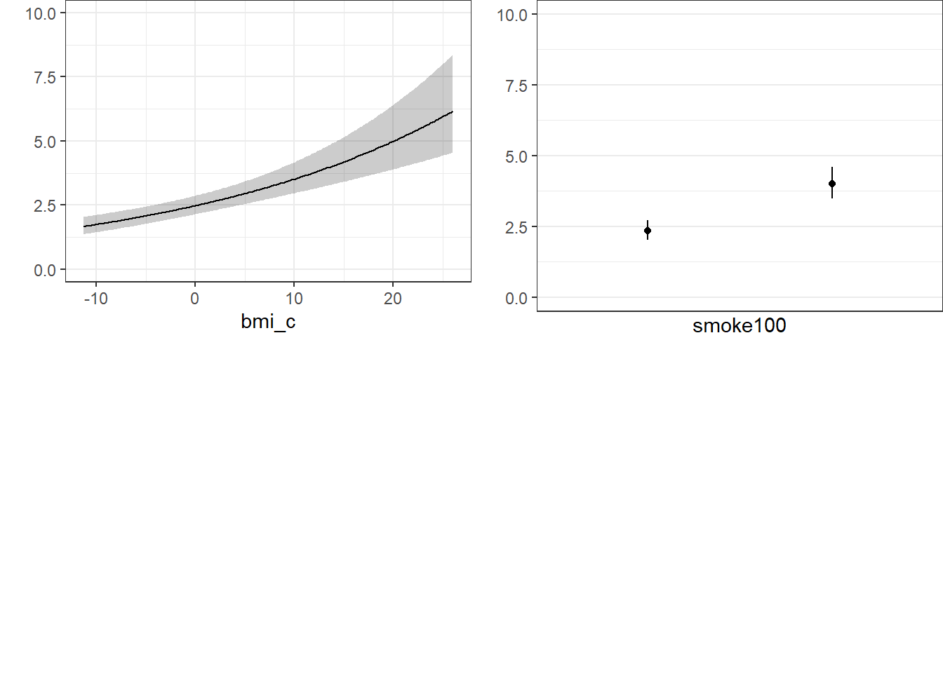

24.11.5 Summary of a Glm fit

summary(mod_poi_od_Glm_1)

             Effects              Response : physhealth 

 Factor   Low     High   Diff.  Effect  S.E.     Lower 0.95 Upper 0.95
 bmi_c    -5.0513 3.6362 8.6875 0.30450 0.048742 0.20891    0.4001    
 smoke100  0.0000 1.0000 1.0000 0.53251 0.098308 0.33971    0.7253    

24.11.6 Plot of the Summary

plot(summary(mod_poi_od_Glm_1))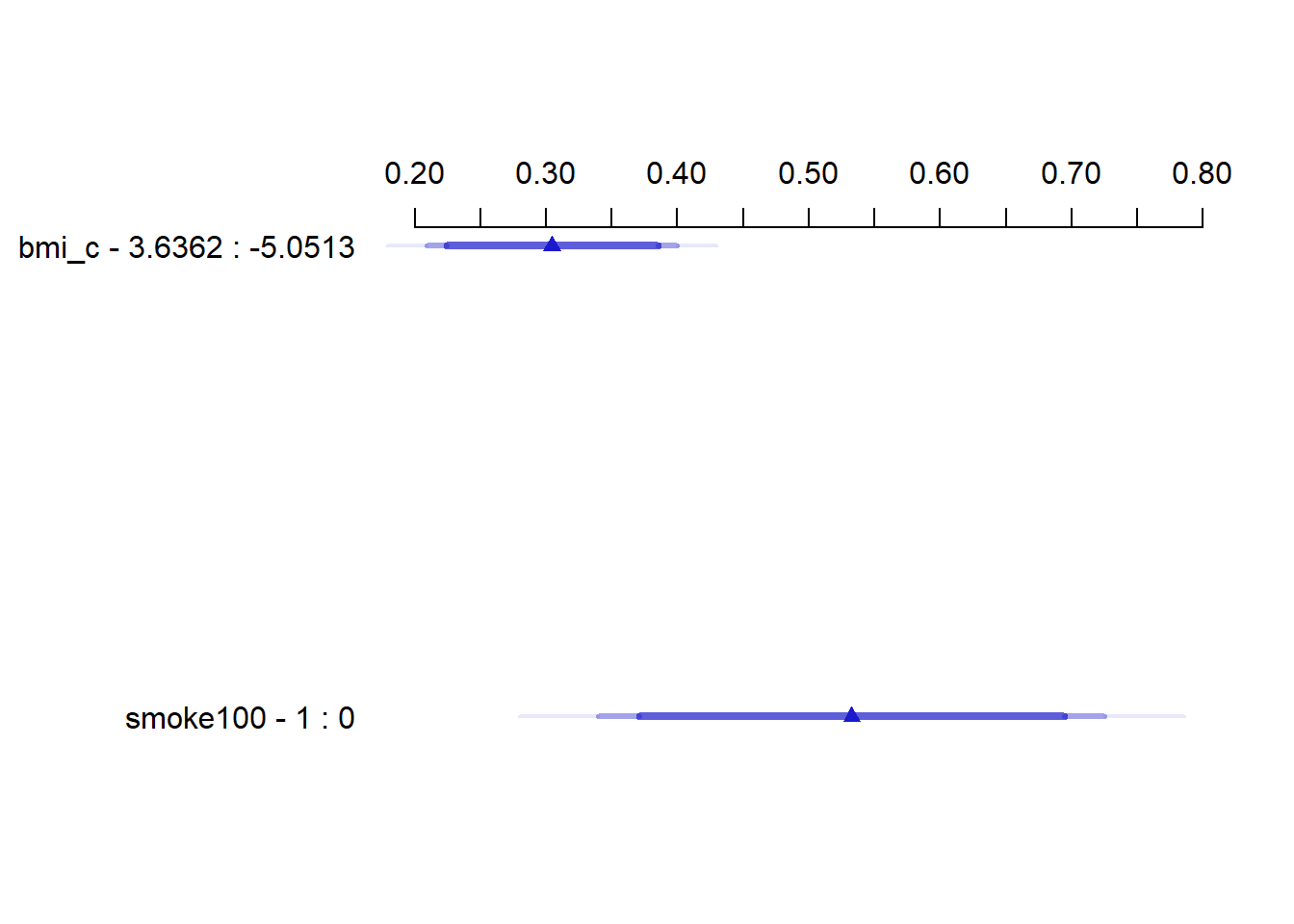

24.11.7 Nomogram of a Glm fit

plot(nomogram(mod_poi_od_Glm_1, fun = exp, 
              funlabel = "physhealth days"))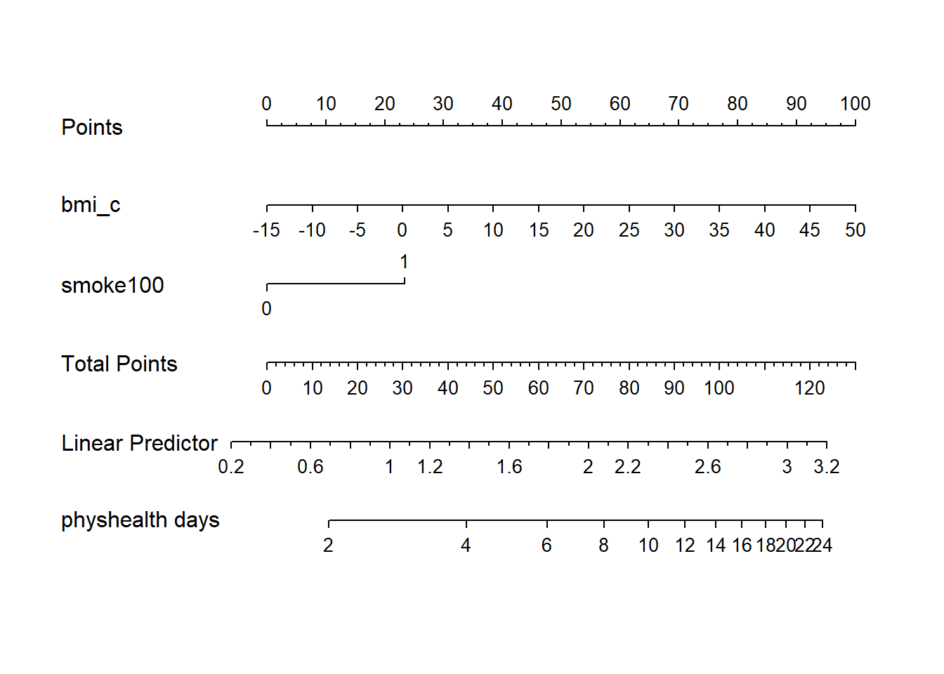

Note the use of fun=exp in both the ggplot of Predict and the nomogram. What’s that doing?

In the next chapter, we’ll expand beyond Poisson regression to consider a Negative Binomial model.

---

1. This discussion is motivated by Section 6.2 of Gelman and Hill.

2. See http://data.library.virginia.edu/getting-started-with-negative-binomial-regression-modeling/

3. See Zeileis A Kleiber C Jackman S Regression Models for Count Data in R Vignette at https://cran.r-project.org/web/packages/pscl/vignettes/countreg.pdf