6  Comparing Two Groups

6.1 R setup for this chapter

Note

Appendix A lists all R packages used in this book, and also provides R session information. Appendix B describes the 431-Love.R script, and demonstrates its use.

library(ggdist)
library(infer)
library(knitr)
library(MKinfer)
library(patchwork)
library(readxl)
library(rstanarm)

library(easystats)
library(tidyverse)

source("data/Love-431.R")
theme_set(theme_bw())

6.2 Comparing Two Groups

In making a choice between two alternatives, questions such as the following become paramount.

• Is there a status quo?
• Is there a standard approach?
• What are the costs of incorrect decisions?
• Are such costs balanced?

The process of comparing the means/medians/proportions/rates of the populations represented by two independently obtained samples can be challenging, and such an approach is not always the best choice. Often, specially designed experiments can be more informative at lower cost (i.e. smaller sample size). As one might expect, using these more sophisticated procedures introduces trade-offs, but the costs are typically small relative to the gain in information.

When faced with such a comparison of two alternatives, a test based on paired data is often much better than a test based on two distinct, independent samples. Why? If we have done our experiment properly, the pairing lets us eliminate background variation that otherwise hides meaningful differences.

6.3 Data from an Excel (.xlsx) file: Parkinson’s Disease Trial

Note

Appendix C provides further guidance on pulling data from other systems into R, while Appendix D gives more information (including download links) for all data sets used in this book.

We will demonstrate ideas in this chapter using a tibble containing information on a simulated trial assessing the effect of lixisenatide (as compared to a placebo) on the progression of motor disability in persons with Parkinson’s disease. This example is motivated by Meissner et al. (2024), but simplifies the study considerably, and uses fake data.

The information we have is gathered in an Excel file called park_rct.xlsx within our data folder. We will use a function from the readxl package in R to help us ingest this information into a tibble called park_rct, using the code below.

park_rct <- read_xlsx("data/park_rct.xlsx") |>
  mutate(across(where(is.character), as_factor)) |>
  mutate(Person = as.character(Person))

park_rct

# A tibble: 152 × 5
   Person Treatment    MDS3_base MDS3_12m MDS3_delta
   <chr>  <fct>            <dbl>    <dbl>      <dbl>
 1 SUB001 Placebo             18       19          1
 2 SUB002 Placebo             21       25          4
 3 SUB003 Lixisenatide         0        0          0
 4 SUB004 Placebo             25       43         18
 5 SUB005 Placebo             22        9        -13
 6 SUB006 Lixisenatide        15        5        -10
 7 SUB007 Lixisenatide        20       30         10
 8 SUB008 Lixisenatide         2        0         -2
 9 SUB009 Placebo             23       32          9
10 SUB010 Lixisenatide        16       16          0
# ℹ 142 more rows

Variables in the park_rct tibble are described below. A reminder that these are fake (simulated) data.

Variable	Description
Person	participant code: ranges from SUB001 to SUB152
Treatment	Placebo or Lixisenatide
MDS3_base	Baseline MDS-UPDRS part III score
MDS3_12m	MDS-UPDRS part III score after 12 months
MDS3_delta	Change (MDS3_12m minus MDS3_base)

The study aims to assess the effect of lixisenatide (vs. placebo) on the progression of motor disability in persons with early (diagnosed less than 3 years) Parkinson’s disease. The primary outcome (end point) of interest for us is the change from baseline in scores on the Movement Disorder Society–Unified Parkinson’s Disease Rating Scale (MDS-UPDRS) part III (range, 0 to 132, with higher scores indicating greater motor disability), which was assessed in patients in the on-medication state at 12 months. More details on the MDS-UPDRS are available at Goetz, Christopher G., et al. (2008).

6.4 Key Questions for Comparing with Independent Samples

Can you answer these questions for our study?

1. What is the population under study?
2. What is the sample? Is it representative of the population?
3. Who are the subjects / individuals within the sample?
4. What data are available on each individual?

6.4.1 RCT Caveats

The placebo-controlled, double-blind randomized clinical trial, especially if pre-registered, is often considered the best feasible study for assessing the effectiveness of a treatment. While that’s not always true, it is a very solid design. The primary caveat is that the patients who are included in such trials are rarely excellent representations of the population of potentially affected patients as a whole.

6.5 Exploratory Data Analysis

We have two independent samples here, where the placebo patients aren’t matched in any way to the Lixisenatide patients. The Lixisenatide group has two more subjects, so the design isn’t (quite) balanced (which would require equal sample sizes in each sample) although it’s close.

6.5.1 Visualizing Two Independent Samples

A common choice for visualizing the distributions of two independent samples is to fit a comparison boxplot. Here, we’ll augment the plot with a violin to show the shape of the distribution, and a red point to indicate the means in each group. We’ll also fill in the colors of the violins with two distinct colors from the “Set2” palette in R¹.

ggplot(park_rct, aes(y = Treatment, x = MDS3_delta, fill = Treatment)) +
  geom_violin() +
  geom_boxplot(width = 0.3, fill = "cornsilk", notch = TRUE) +
  stat_summary(fun = mean, geom = "point", size = 2, col = "red") +
  scale_fill_brewer(palette = "Set2") +
  guides(fill = "none")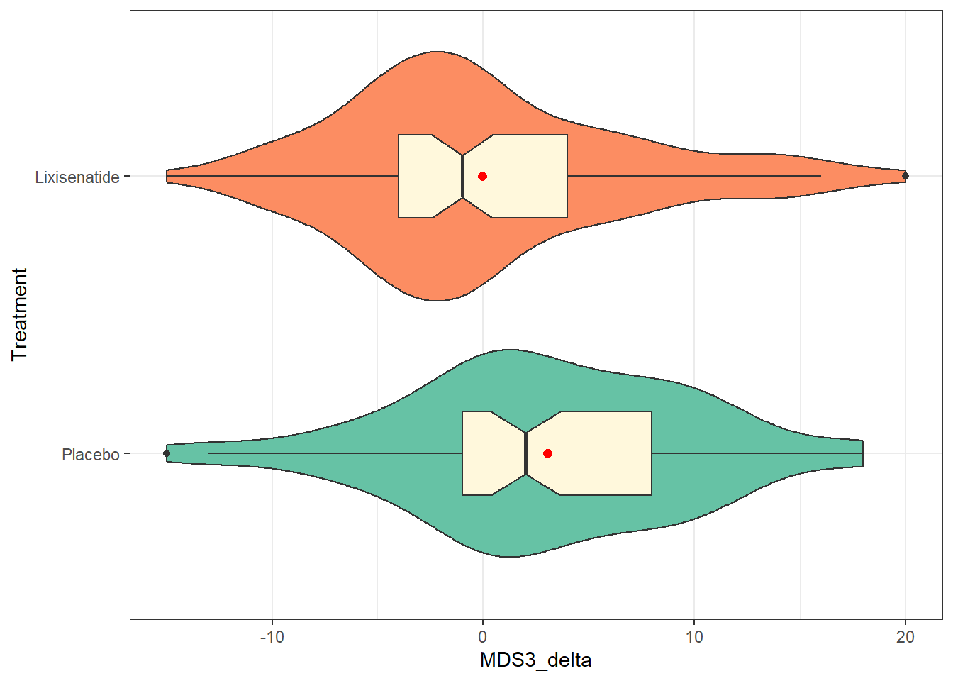

Another approach we might consider is the use of stat_slab() and slat_dotsinterval() from the ggdist package to simultaneously display:

• a smoothed histogram of the data’s distribution,
• a rain cloud plot showing the distribution in a dotplot, and
• a line with a point showing the median of the data along with (by default) changes in line size which indicate 66% and 95% intervals for the data.

ggplot(park_rct, aes(y = Treatment, x = MDS3_delta, fill = Treatment)) +
  stat_slab(aes(thickness = after_stat(pdf * n)), scale = 0.7) +
  stat_dotsinterval(side = "bottom", scale = 0.7, slab_linewidth = NA) +
  scale_fill_brewer(palette = "Set2") +
  guides(fill = "none") +
  theme_bw()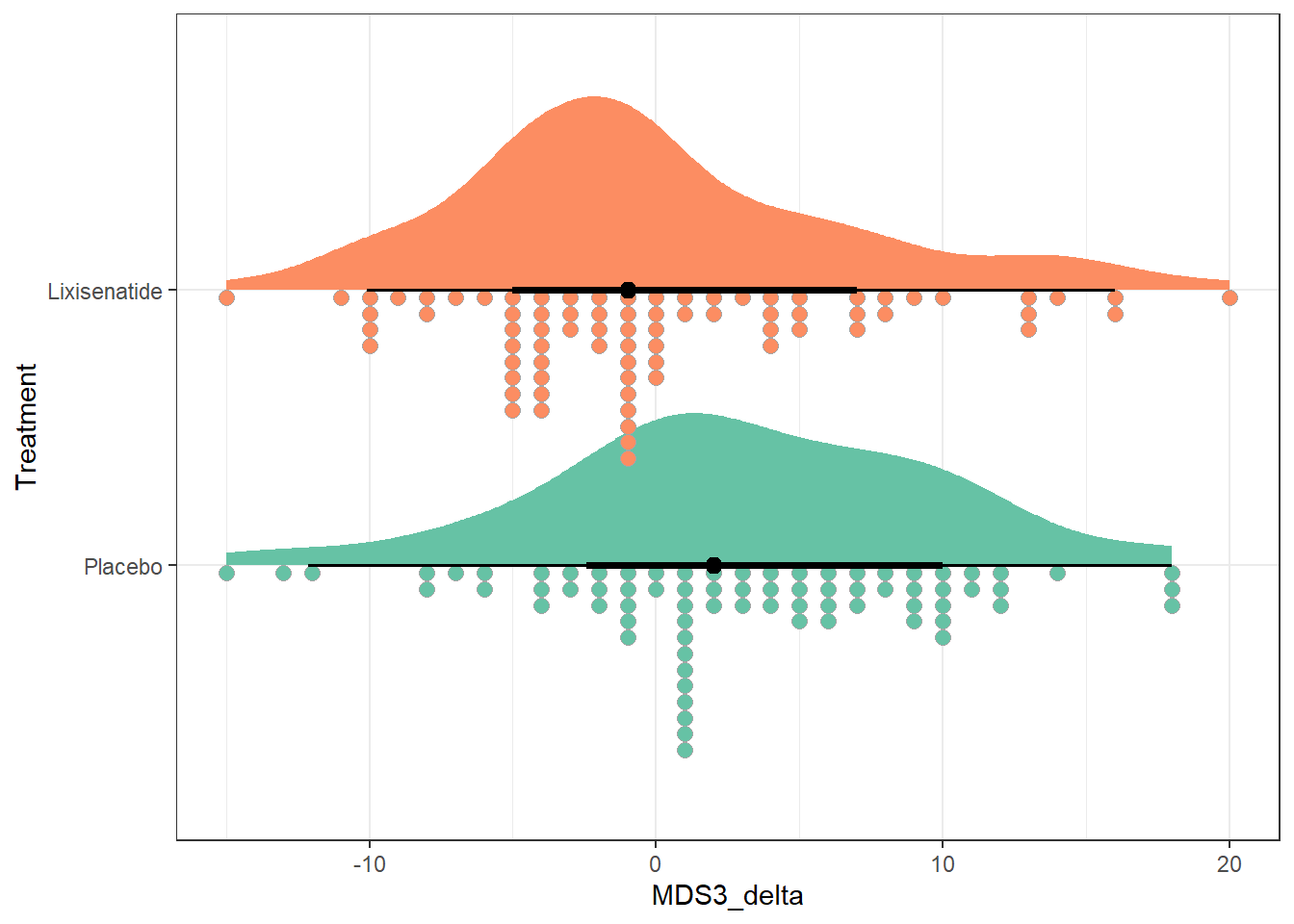

Finally, we show separate Normal Q-Q plots of each of the two treatment groups, joined together using the patchwork package into a single figure. Most of the points in each treatment group track with the expectations of a Normal distribution, as indicated by the red line being a reasonably good fit to the data.

p1 <- park_rct |>
  filter(Treatment == "Lixisenatide") |>
  ggplot(aes(sample = MDS3_delta)) +
  geom_qq() +
  geom_qq_line(col = "red") +
  labs(y = "Lixisenatide", x = "Standard Normal")

p2 <- park_rct |>
  filter(Treatment == "Placebo") |>
  ggplot(aes(sample = MDS3_delta)) +
  geom_qq() +
  geom_qq_line(col = "red") +
  labs(y = "Placebo", x = "Standard Normal")

p1 + p2 +
  plot_annotation(title = "Normal Q-Q plots of MDS3_delta")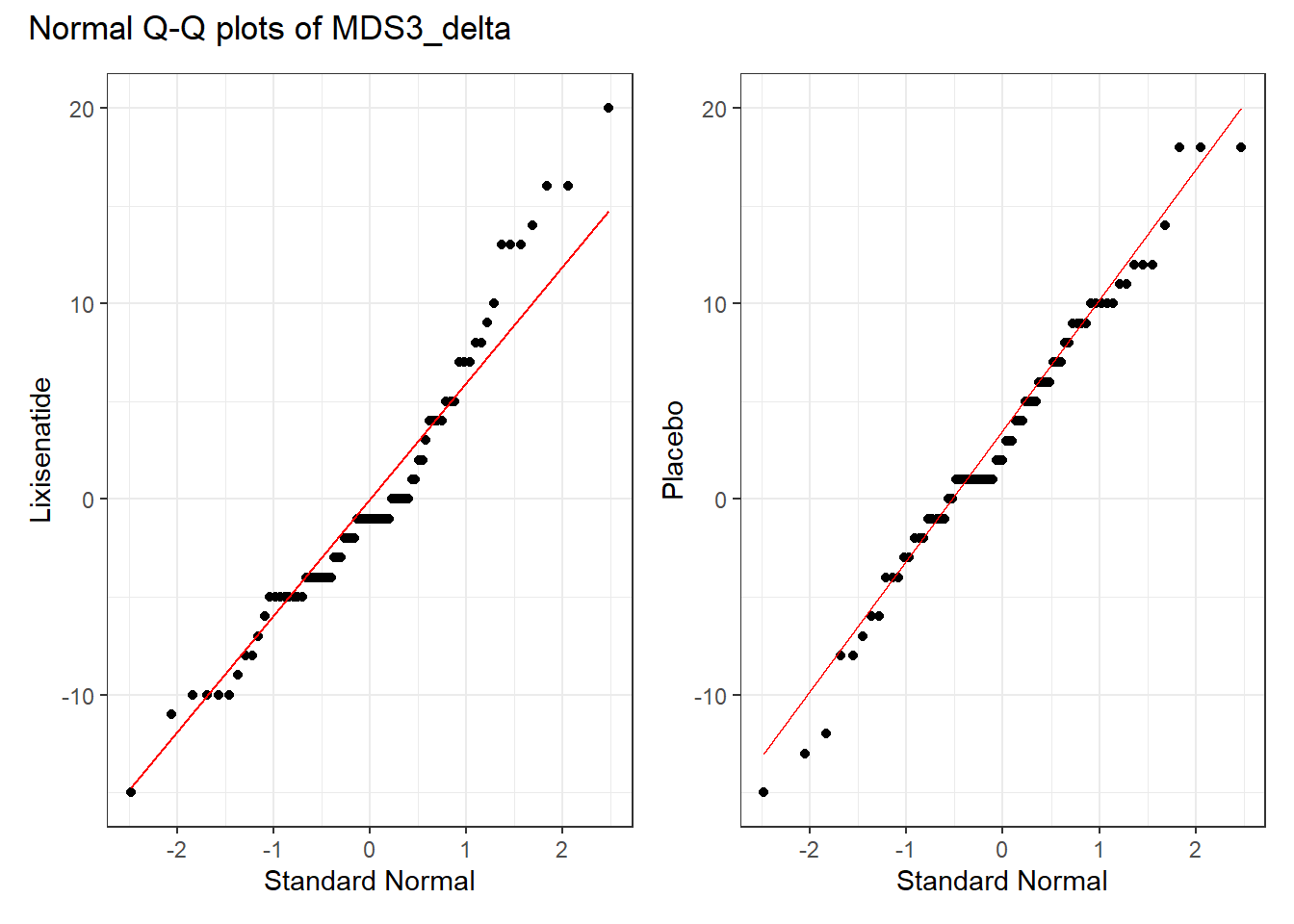

6.5.2 Numerical Summaries

park_rct |>
  reframe(lovedist(MDS3_delta), .by = Treatment) |>
  kable(digits = 2)

Treatment	n	miss	mean	sd	med	mad	min	q25	q75	max
Placebo	75	0	3.04	6.84	2	5.93	-15	-1	8	18
Lixisenatide	77	0	-0.04	6.93	-1	5.93	-15	-4	4	20

We see that the mean change in the placebo group is about 3 points on the scale, indicating somewhat higher motor disability at 12 months than at baseline for those subjects. In the Lixisenatide group, we have a slightly negative mean change very close to zero (the median is -1) indicating that the subjects in that group have (very) slightly lower disability at 12 months than they did at baseline. So the direction of the effect we’re seeing appears to be somewhat favorable for Lixisenatide as compared to placebo, at least in terms of the point estimate of the difference in means.

How much uncertainty do we have in those estimates? One way to start thinking about that is to think about the variation within each group. Our measures of spread shown above appear fairly similar across the two treatment groups, in terms of standard deviations (6.8 vs. 6.9), MAD (both 5.9) and even the interquartile range (IQR).

6.6 Using a linear model

To start, we’ll build a 95% confidence interval for the difference in treatment means using a linear model, with the outcome MDS3_delta being predicted by the Treatment group.

fit1 <- lm(MDS3_delta ~ Treatment, data = park_rct)

fit1

Call:
lm(formula = MDS3_delta ~ Treatment, data = park_rct)

Coefficients:
          (Intercept)  TreatmentLixisenatide  
                3.040                 -3.079  

The model equation is MDS3_delta = 3.04 - 3.08 (Treatment = Lixisenatide), which implies that the model estimates that:

• subjects on placebo will have MDS3_delta of 3.04, on average.
• subjects on Lixisenatide will have MDS3_delta of 3.04 - 3.08 = -0.04, on average.

and of course, these are just the sample means in each group.

Here’s one more detailed summary of this fit.

summary(fit1)

Call:
lm(formula = MDS3_delta ~ Treatment, data = park_rct)

Residuals:
    Min      1Q  Median      3Q     Max 
-18.040  -4.040  -0.961   4.039  20.039 

Coefficients:
                      Estimate Std. Error t value Pr(>|t|)    
(Intercept)             3.0400     0.7951   3.824 0.000192 ***
TreatmentLixisenatide  -3.0790     1.1171  -2.756 0.006573 ** 
---
Signif. codes:  0 '***' 0.001 '**' 0.01 '*' 0.05 '.' 0.1 ' ' 1

Residual standard error: 6.886 on 150 degrees of freedom
Multiple R-squared:  0.0482,    Adjusted R-squared:  0.04186 
F-statistic: 7.597 on 1 and 150 DF,  p-value: 0.006573

We’ll note that the Multiple R-squared statistic indicates that the predictors in this model (here we have only Treatment as a predictor) account for about 4.8% of the variation in our outcome (MDS3_delta) using this linear model.

6.6.1 Obtaining t-based confidence intervals

One way to obtain confidence intervals for the coefficients in our fit1 model is to use the confint() function to obtain confidence intervals using the t distribution.

confint(fit1, level = 0.95)

                          2.5 %     97.5 %
(Intercept)            1.468992  4.6110084
TreatmentLixisenatide -5.286228 -0.8716937

The point estimate of the (Lixisenatide - Placebo) treatment effect is -3.08, with 95% CI (-5.29, -0.87).

Another way (and this is my usual approach nowadays) to obtain these results is to use model_parameters() as applied to our fitted model, fit1.

fit1 |>
  model_parameters(ci = 0.95) |>
  kable(digits = 2)

Parameter	Coefficient	SE	CI	CI_low	CI_high	t	df_error	p
(Intercept)	3.04	0.80	0.95	1.47	4.61	3.82	150	0.00
TreatmentLixisenatide	-3.08	1.12	0.95	-5.29	-0.87	-2.76	150	0.01

If we like, we can also obtain and present contrasts from the model as follows. In this relatively simple case, all of these approaches give the same conclusions.

cons <- estimate_contrasts(fit1, contrast = "Treatment", ci = 0.95)
cons |> kable(digits = 2)

Level1	Level2	Difference	CI_low	CI_high	SE	df	t	p
Placebo	Lixisenatide	3.08	0.87	5.29	1.12	150	2.76	0.01

6.6.2 Obtaining bootstrapped confidence intervals

So far, we have produced t-based confidence intervals for the coefficients in model fit1. We could also bootstrap the confidence interval for the difference in means shown by our linear model with the following augmentations to the model_parameters() command.

set.seed(43123)

model_parameters(fit1, bootstrap = TRUE, iterations = 2000,
  ci = 0.95, centrality = "median", ci_method = "quantile")

Parameter                | Coefficient |         95% CI |      p
----------------------------------------------------------------
(Intercept)              |        3.03 | [ 1.42,  4.55] | < .001
Treatment [Lixisenatide] |       -3.07 | [-5.21, -0.82] | 0.009 

Uncertainty intervals (equal-tailed) are naıve bootstrap intervals.

The resulting estimate still describes a difference in means, but it shows the median result of that difference across 2000 bootstrapped samples. We see now that our estimated effect of Lixisenatide as compared to Placebo is -3.07 points on the MDS3_delta scale, with a 95% confidence interval stretching from (-5.21, -0.82). Note, too, that we set a random seed here to allow us to replicate the results.

6.7 t test for Two Independent Samples

6.7.1 Assuming equal population variances

If we assume equal population variances, a t test produces identical results to our linear model fit1, as demonstrated below.

fit2 <- t.test(MDS3_delta ~ Treatment,
  data = park_rct, var.equal = TRUE)

fit2 |>
  model_parameters(ci = 0.95) |>
  kable(digits = 2)

Parameter	Group	Mean_Group1	Mean_Group2	Difference	CI	CI_low	CI_high	t	df_error	p	Method	Alternative
MDS3_delta	Treatment	3.04	-0.04	3.08	0.95	0.87	5.29	2.76	150	0.01	Two Sample t-test	two.sided

6.7.2 Cohen’s d assuming equal population variances

We can also produce an estimate of Cohen’s d statistic while assuming equal variances (i.e. making use of a pooled t test.)

cohens_d(MDS3_delta ~ Treatment, data = park_rct, pooled_sd = TRUE)

Cohen's d |       95% CI
------------------------
0.45      | [0.12, 0.77]

- Estimated using pooled SD.

Cohen’s d estimates the standardized difference between the mean MDS3_delta scores across the two Treatment groups. Here, we have a value of 0.45 with a 95% CI of (0.12, 0.77).

This Cohen’s d indicates that the differences between the means are approximately 45% of the size (on average) as their pooled standard deviation. As we’ve seen, the general guidelines for interpreting this effect size suggested by Cohen (1988) are:

• 0.2 indicates a small effect
• 0.5 indicates a moderate effect
• 0.8 indicates a large effect

So our observed d = 0.45 indicates a small to moderate difference from 0.

6.7.3 Estimated without pooling the standard deviation

We can also estimate the confidence interval without assuming equal population variances (i.e. without pooling the standard deviation) across our two Treatments. This is actually the default t.test() approach in R, and the code looks like this:

fit3 <- t.test(MDS3_delta ~ Treatment, data = park_rct)

fit3 |>
  model_parameters(ci = 0.95) |>
  kable(digits = 2)

Parameter	Group	Mean_Group1	Mean_Group2	Difference	CI	CI_low	CI_high	t	df_error	p	Method	Alternative
MDS3_delta	Treatment	3.04	-0.04	3.08	0.95	0.87	5.29	2.76	149.97	0.01	Welch Two Sample t-test	two.sided

Our new 95% confidence interval using this Welch two-sample t test procedure is (0.87, 5.29) for the size of the Placebo - Lixisenatide difference. The Cohen’s d estimate of the standardized difference in means can also be obtained while not assuming a pooled standard deviation using the following code.

cohens_d(MDS3_delta ~ Treatment, data = park_rct, pooled_sd = FALSE)

Cohen's d |       95% CI
------------------------
0.45      | [0.12, 0.77]

- Estimated using un-pooled SD.

Note that this result doesn’t change materially as compared to the Cohen’s d when assuming equal variances in the two Treatment groups and this is because:

1. The sample sizes in the two Treatment groups are quite close, and
2. The sample standard deviations in the two Treatment groups are also quite similar.

6.8 Bayesian linear regression

Let’s now fit a linear model to describe the difference in MDS3_delta between the two Treatment groups, using a Bayesian approach with the default choice of prior, which is weakly informative.

set.seed(431)
fit4 <- stan_glm(MDS3_delta ~ Treatment, data = park_rct, refresh = 0)

## refresh = 0 avoids printing the iteration updates

post4 <- describe_posterior(fit4, ci = 0.95)

print_md(post4, digits = 2)

Summary of Posterior Distribution

Parameter	Median	95% CI	pd	ROPE	% in ROPE	Rhat	ESS
(Intercept)	3.03	[ 1.48, 4.54]	100%	[-0.70, 0.70]	0%	0.999	4143.00
TreatmentLixisenatide	-3.08	[-5.30, -0.85]	99.72%	[-0.70, 0.70]	0%	1.000	4181.00

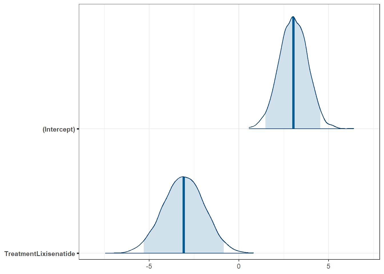
Our estimate of the difference in means between the two treatment groups is -3.08 with a 95% credible interval ranging between (-5.30, -0.85). We note again that this is essentially the same conclusion that we drew from the t test approach.

The difference here is that the model produces a credible interval rather than a confidence interval, which changes (a bit) the nature of what we can conclude about that interval.

Specifically, we could now conclude that there is a 95% chance that the true value of the difference in means between the Treatment groups is in the range (-5.30, -0.85), but only if we were willing to assume that the prior distribution we established for the difference in means was appropriate.

Moreover, from the pd result, we estimate a 99.72% chance that the true difference in means is in the direction we have observed in this model (that Lixisenatide does better than Placebo), and that with a default choice of minimal practical effect size (as shown by the ROPE and % in ROPE materials) that there is almost no chance that the effects is ignorably small.

We can show some graphs of the simulated results from our posterior distribution of our model’s coefficients, for example…

plot(fit4, plotfun = "areas", prob = 0.95,
  pars = c("(Intercept)", "TreatmentLixisenatide"))

And we can summarize the Bayesian fit with the model_parameters() command as follows:

fit4 |>
  model_parameters() |>
  kable(digits = 2)

Parameter	Median	CI	CI_low	CI_high	pd	Rhat	ESS	Prior_Distribution	Prior_Location	Prior_Scale
(Intercept)	3.03	0.95	1.48	4.54	1	1	4143.11	normal	1.48	17.59
TreatmentLixisenatide	-3.08	0.95	-5.30	-0.85	1	1	4180.84	normal	0.00	35.06

The nice part of this last bit of output is that it displays the actual prior distributions assumed for each coefficient (both the intercept and the treatment effect.)

6.9 Using the Bootstrap

6.9.1 Bootstrap CI for Means

We can use the approach available in the infer package demonstrated below to obtain a 95% percentile bootstrap confidence interval for the difference in means between the two Treatment groups as follows. Note the need to set a random seed for replicability.

set.seed(431)
park_rct |>
  specify(MDS3_delta ~ Treatment) |>
  generate(reps = 1000, type = "bootstrap") |>
  calculate(stat = "diff in means",
    order = c("Placebo", "Lixisenatide") ) |>
  get_confidence_interval(level = 0.95, type = "percentile")

# A tibble: 1 × 2
  lower_ci upper_ci
     <dbl>    <dbl>
1    0.809     5.36

Again, we have a fairly similar estimated confidence interval (0.81, 5.36) to the ones we saw previously.

Another approach to doing essentially the same thing is available through the boot.t.test() function in the MKinfer package, as follows:

set.seed(431)
boot.t.test(MDS3_delta ~ Treatment, var.equal = TRUE, R = 2000,
  data = park_rct, conf.level = 0.95)

    Bootstrap Two Sample t-test

data:  MDS3_delta by Treatment
number of bootstrap samples:  2000
bootstrap p-value = 0.008 
bootstrap difference of means (SE) = 3.102324 (1.134524) 
95 percent bootstrap percentile confidence interval:
 0.9155498 5.2608788

Results without bootstrap:
t = 2.7562, df = 150, p-value = 0.006573
alternative hypothesis: true difference in means is not equal to 0
95 percent confidence interval:
 0.8716937 5.2862284
sample estimates:
     mean in group Placebo mean in group Lixisenatide 
                3.04000000                -0.03896104 

If we want to run the bootstrapped t test without assuming equal population variances, we can adapt the boot.t.test() function accordingly, like this:

set.seed(431)
boot.t.test(MDS3_delta ~ Treatment, var.equal = FALSE, R = 4000,
  data = park_rct, conf.level = 0.95)

    Bootstrap Welch Two Sample t-test

data:  MDS3_delta by Treatment
number of bootstrap samples:  4000
bootstrap p-value = 0.009 
bootstrap difference of means (SE) = 3.074508 (1.107546) 
95 percent bootstrap percentile confidence interval:
 0.8585108 5.2140563

Results without bootstrap:
t = 2.7567, df = 149.97, p-value = 0.006564
alternative hypothesis: true difference in means is not equal to 0
95 percent confidence interval:
 0.872082 5.285840
sample estimates:
     mean in group Placebo mean in group Lixisenatide 
                3.04000000                -0.03896104 

Again, our results stay similar to what we’ve seen in the past.

6.9.2 Bootstrap CI for Medians

We might also want to find a bootstrap confidence interval for the difference in medians rather than means across the two Treatment groups. We saw earlier that the median MDS3_delta in the Placebo group was +2 and the median in the Lixisenatide group was -1, a difference of 3 points on the MDS3_delta scale. The following code from the infer package is a reasonable choice to obtain a bootstrap for this difference in medians.

set.seed(431)
park_rct |>
  specify(MDS3_delta ~ Treatment) |>
  generate(reps = 2500, type = "bootstrap") |>
  calculate(stat = "diff in medians", 
            order = c("Placebo", "Lixisenatide") ) |>
  get_ci(level = 0.95, type = "percentile")

# A tibble: 1 × 2
  lower_ci upper_ci
     <dbl>    <dbl>
1        2      6.5

All of our previous estimates have focused on a difference in means, while this instead finds a difference in medians - and this explains some of the difference we observe.

6.10 Wilcoxon Rank Sum Test

Finally, you may wish to run a Wilcoxon rank sum test. This test compares the locations without using either the mean or the median of the original differences, but instead first ranks the observed MDS3_delta values regardless of Treatment group, and then compares the centers (locations) of those distributions. Here’s how you could obtain this test (and 95% confidence interval) in R.

wilcox.test(MDS3_delta ~ Treatment, data = park_rct, exact = FALSE,
  conf.int = TRUE, conf.level = 0.95)

    Wilcoxon rank sum test with continuity correction

data:  MDS3_delta by Treatment
W = 3789.5, p-value = 0.0008758
alternative hypothesis: true location shift is not equal to 0
95 percent confidence interval:
 1.999936 5.999975
sample estimates:
difference in location 
              3.999955 

Of course, these results aren’t describing either the difference in means or the difference in medians of the treatment groups on our outcome, so they’re meaningfully harder to think about.

6.11 Our Results

In this study, we compared the MDS3_delta levels across two Treatment groups (Lixisenatide and Placebo), obtaining a series of 95% uncertainty intervals. Specifically, we found the following results (in each case using “Lixisenatide - Placebo” as the order for our difference, so that negative values (which indicate less motor disability) are good news for the Lixisenatide drug.

Method	Point Est.	95% Uncertainty Interval	What do we estimate?
linear fit with lm()	-3.08	(-5.29, -0.87)	diff. in means
bootstrap CI after lm() fit	-3.07	(-5.21, -0.82)	diff. in means
pooled t test	-3.08	(-5.29, -0.87)	diff. in means, same as lm()
Welch test	-3.08	(-5.29, -0.87)	diff. in means, unpooled std. dev.
Bayesian fit	-3.08	(-5.30, -0.85)	diff. in means, credible interval
percentile bootstrap	-3.08	(-5.36, -0.81)	diff. in means
bootstrap, pooled sd	-3.10	(-5.26, -0.92)	diff. in means
bootstrap, unpooled sd	-3.07	(-5.21, -0.86)	diff. in means
bootstrap, medians	-3	(-6.5, -2)	diff. in medians

None of these look wildly different from any of the others, and this is mostly because of the following four reasons:

• the sample size is similar in each Treatment group,
• the sample variance is similar in each Treatment group,
• the difference in means across the two Treatment groups is similar to the difference in medians we observe here,
• the distribution of MDS3_delta is fairly similar in each Treatment group, and in both cases is fairly well approximated by a Normal distribution, and
• we used a weakly informative prior distribution in our Bayesian models.

6.12 Paired vs. Independent Samples

One area that consistently trips students up in this course is the thought process involved in distinguishing studies comparing means that should be analyzed using dependent (i.e. paired or matched) samples (as we discussed in Chapter 5) and those which should be analyzed using independent samples (as we discussed in this chapter.)

A paired samples analysis uses additional information about the sample to pair/match subjects receiving the various exposures. That additional information is not part of an independent samples analysis (unpaired testing situation.) The reasons to do this are to (a) increase statistical power, and/or (b) reduce the effect of confounding.

1. In the design of experiments, blocking is the term often used for the process of arranging subjects into groups (blocks) that are similar to one another. Typically, a blocking factor is a source of variability that is not of primary interest to the researcher An example of a blocking factor might be the sex of a patient; by blocking on sex, this source of variability is controlled for, thus leading to greater accuracy.

2. If the sample sizes are not balanced (not equal), the samples must be treated as independent, since there would be no way to precisely link all subjects. So, if we have 10 subjects receiving exposure A and 12 subjects receiving exposure B, a paired samples analysis (such as a paired t test) is not correct.

3. The key element is a meaningful link between each observation in one exposure group and a specific observation in the other exposure group. Given a balanced design, the most common strategy indicating paired samples involves two or more repeated measures on the same subjects. For example, if we are comparing outcomes before and after the application of an exposure, and we have, say, 20 subjects who provide us data both before and after the exposure, then the comparison of results before and after exposure should use a paired samples analysis. The link between the subjects is the subject itself - each exposed subject serves as its own control.

4. The second most common strategy indicating paired samples involves deliberate matching of subjects receiving the two exposures. A matched set of observations (often a pair, but it could be a trio or quartet, etc.) is determined using baseline information and then (if a pair is involved) one subject receives exposure A while the other member of the pair receives exposure B, so that by calculating the paired difference, we learn about the effect of the exposure, while controlling for the variables made similar across the two subjects by the matching process.

5. In order for a paired samples analysis to be used, we need (a) a link between each observation across the exposure groups based on the way the data were collected, and (b) a consistent measure (with the same units of measurement) so that paired differences can be calculated and interpreted sensibly.

If the samples are collected to facilitate a dependent samples analysis, the correlation of the outcome measurements across the groups will often be moderately strong and positive. If that’s the case, then the use of a dependent samples analysis will reduce the effect of baseline differences between the exposure groups, and thus provide a more precise estimate. But even if the correlation is quite small, a dependent samples analysis should provide a more powerful estimate of the impact of the exposure on the outcome than would an independent samples analysis with the same number of observations.

6.13 Summary: Specifying A Two-Sample Study Design

These questions will help specify the details of the study design involved in any comparison of two populations on a quantitative outcome, perhaps with means.

1. What is the outcome under study?
2. What are the (in this case, two) treatment/exposure groups?
3. Were the data collected using matched / paired samples or independent samples?
4. Are the data a random sample from the population(s) of interest? Or is there at least a reasonable argument for generalizing from the sample to the population(s)?
5. What is the confidence level we require here?
6. Are we doing one-sided or two-sided testing/confidence interval generation?
7. If we have paired samples, did pairing help reduce nuisance variation?
   • Also, if we have paired samples, what does the distribution of sample paired differences tell us about which inferential procedure to use?
8. If we have independent samples, what does the distribution of each individual sample tell us about which inferential procedure to use?

6.14 For More Information

1. Chapter 20 of Introduction to Modern Statistics (Çetinkaya-Rundel and Hardin 2024) does a great job discussing the application of point estimates and confidence intervals in the case of two independent samples, using a randomization test, as well as the t-test and bootstrap approaches shown in this chapter.

2. The infer package website has a lot more on methods for performing statistical inference of the type we discuss here, especially the bootstrap approaches.

3. Should you need the formula for the t test comparing two independent samples, I encourage you to look at Wikipedia’s page on Student’s t test in the two-sample t-tests section.

4. Similarly, you could consider the Wikipedia page on the Wilcoxon signed rank test for an example or two and relevant formulas.

5. The Factors chapter and the Spreadsheets chapter in (Wickham, Çetinkaya-Rundel, and Grolemund 2024) can be helpful in extending your understanding of some of the things I’ve done in this chapter.

6. The Get Started with Bayesian Analysis vignette from the easystats family of packages (Makowski, Ben-Shachar, and Lüdecke 2019) is extremely helpful and includes some nice examples.

Çetinkaya-Rundel, Mine, and Johanna Hardin. 2024. Introduction to Modern Statistics. Second Edition. OpenIntro Project. https://openintro-ims.netlify.app/.

Cohen, Jacob. 1988. Statistical Power Analysis for the Behavioral Sciences. 2nd ed. New York: Routledge. https://www.utstat.toronto.edu/~brunner/oldclass/378f16/readings/CohenPower.pdf.

Goetz, Christopher G., et al. 2008. “MDS-Unified Parkinson’s Disease Rating Scale (MDS-UPDRS).” https://www.movementdisorders.org/MDS/MDS-Rating-Scales/MDS-Unified-Parkinsons-Disease-Rating-Scale-MDS-UPDRS.htm.

Makowski, Dominique, Mattan S. Ben-Shachar, and Daniel Lüdecke. 2019. “bayestestR: Describing Effects and Their Uncertainty, Existence and Significance Within the Bayesian Framework.” Journaal of Open Source Software 4 (40): 1541. https://doi.org/doi.org/10.21105/joss.01541.

Meissner, Wassilios G., Philippe Remy, Caroline Giordana, David Maltête, Pascal Derkinderen, Jean-Luc Houéto, and Mathieu Anheim for the LIXIPARK Study Group. 2024. “Trial of Lixisenatide in Early Parkinson’s Disease.” The New England Journal of Medicine 390 (13): 1176–85. https://doi.org/10.1056/NEJMoa2312323.

Wickham, Hadley, Mine Çetinkaya-Rundel, and Garrett Grolemund. 2024. “R for Data Science, 2e.” https://r4ds.hadley.nz/.

---

1. Emil Hvitfeldt provides a nearly comprehensive list of palettes in R here if you’re interested.