19 Multiple Regression and Model Selection
19.1 R setup for this chapter
Appendix A lists all R packages used in this book, and also provides R session information.
19.2 Data is bodyfat
Appendix C provides further guidance on pulling data from other systems into R, while Appendix D gives more information (including download links) for all data sets used in this book.
My source for these data was Kaggle, although the data have been published in several other places. The data describe 252 men whose percentage of body fat was determined via underwater weighing and Siri’s (1956) equation.
From Kaggle:
These data are used to produce the predictive equations for lean body weight given in the abstract “Generalized body composition prediction equation for men using simple measurement techniques”, K.W. Penrose, A.G. Nelson, A.G. Fisher, FACSM, Human Performance Research Center, Brigham Young University, Provo, Utah 84602 as listed in Medicine and Science in Sports and Exercise, vol. 17, no. 2, April 1985, p. 189.
bodyfat <- read_csv("data/bodyfat.csv", show_col_types = FALSE) |>
  janitor::clean_names()

bodyfat
# A tibble: 248 × 16
kag_row density siri_bf age weight height neck chest abdomen hip thigh
<chr> <dbl> <dbl> <dbl> <dbl> <dbl> <dbl> <dbl> <dbl> <dbl> <dbl>
1 sub_001 1.07 12.3 23 154. 67.8 36.2 93.1 85.2 94.5 59
2 sub_002 1.09 6.1 22 173. 72.2 38.5 93.6 83 98.7 58.7
3 sub_003 1.04 25.3 22 154 66.2 34 95.8 87.9 99.2 59.6
4 sub_004 1.08 10.4 26 185. 72.2 37.4 102. 86.4 101. 60.1
5 sub_005 1.03 28.7 24 184. 71.2 34.4 97.3 100 102. 63.2
6 sub_006 1.05 21.3 24 210. 74.8 39 104. 94.4 108. 66
7 sub_007 1.05 19.2 26 181 69.8 36.4 105. 90.7 100. 58.4
8 sub_008 1.07 12.4 25 176 72.5 37.8 99.6 88.5 97.1 60
9 sub_009 1.09 4.1 25 191 74 38.1 101. 82.5 99.9 62.9
10 sub_010 1.07 11.7 23 198. 73.5 42.1 99.6 88.6 104. 63.1
# ℹ 238 more rows
# ℹ 5 more variables: knee <dbl>, ankle <dbl>, biceps <dbl>, forearm <dbl>,
# wrist <dbl>The variables included are:
| Variable | Description1 |
|---|---|
kag_row |
subject identification code |
density |
density determined from underwater weighing |
siri_bf |
percent body fat from Siri’s (1956) equation2 |
age |
age (years) |
weight |
weight (pounds) |
height |
height (inches) |
neck |
neck circumference (cm) |
chest |
chest circumference (cm) |
abdomen |
abdomen circumference (cm) |
hip |
hip circumference (cm) |
thigh |
thigh circumference (cm) |
knee |
knee circumference (cm) |
ankle |
ankle circumference (cm) |
biceps |
biceps (extended) circumference (cm) |
forearm |
forearm circumference (cm) |
wrist |
wrist circumference (cm) |
As Kaggle motivates,
Accurate measurement of body fat is inconvenient/costly and it is desirable to have easy methods of estimating body fat that are not inconvenient/costly.
So our job will be to predict the siri_bf measure using a well-chosen subset of the 13 predictors listed above from age through wrist.
Model selection is a very big and somewhat controversial topic - we’re just touching on a couple of semi-useful tools here, but there are lots of situations where semi-automated techniques for model selection like those I will discuss in this chapter do not work well, and quite a few others where they are actively bad choices.
Note that we have no missing data here to worry about.
n_miss(bodyfat)[1] 019.3 Need for transformation?
We’ll start by considering whether the Box-Cox approach suggests any particular transformation for our outcome variable when we fit a kitchen sink model (e.g., a model including main effects of all available predictors.)
fit1 <- lm(
  siri_bf ~ age + weight + height + neck + chest +
    abdomen + hip + thigh + knee + ankle + biceps +
    forearm + wrist,
  data = bodyfat
)

boxCox(fit1)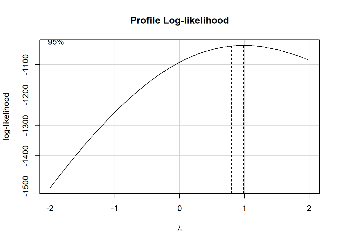
Since the recommended power transformation parameter \(\lambda\) is quite close to 1, we’ll not be using any transformation in this chapter.
19.4 The Full OLS model
model_parameters(fit1, ci = 0.95)Parameter | Coefficient | SE | 95% CI | t(234) | p
---------------------------------------------------------------------
(Intercept) | -14.73 | 22.35 | [-58.77, 29.30] | -0.66 | 0.510
age | 0.05 | 0.03 | [ -0.01, 0.11] | 1.53 | 0.128
weight | -0.09 | 0.06 | [ -0.21, 0.04] | -1.40 | 0.162
height | -0.08 | 0.18 | [ -0.44, 0.27] | -0.46 | 0.644
neck | -0.48 | 0.23 | [ -0.94, -0.02] | -2.06 | 0.040
chest | -0.03 | 0.10 | [ -0.23, 0.18] | -0.27 | 0.786
abdomen | 0.97 | 0.09 | [ 0.79, 1.14] | 10.69 | < .001
hip | -0.21 | 0.15 | [ -0.50, 0.08] | -1.45 | 0.148
thigh | 0.20 | 0.15 | [ -0.09, 0.49] | 1.36 | 0.176
knee | 0.04 | 0.25 | [ -0.45, 0.52] | 0.14 | 0.886
ankle | 0.17 | 0.22 | [ -0.27, 0.61] | 0.78 | 0.436
biceps | 0.16 | 0.17 | [ -0.18, 0.50] | 0.93 | 0.354
forearm | 0.44 | 0.20 | [ 0.05, 0.83] | 2.21 | 0.028
wrist | -1.59 | 0.53 | [ -2.64, -0.54] | -2.98 | 0.003
Uncertainty intervals (equal-tailed) and p-values (two-tailed) computed
using a Wald t-distribution approximation.check_model(fit1)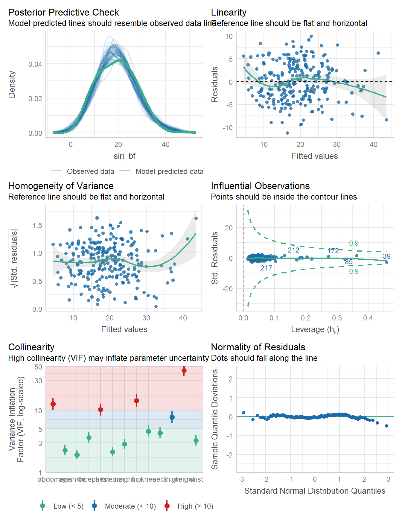
It looks like we have several variables here with very high collinearity.
model_performance(fit1)# Indices of model performance
AIC | AICc | BIC | R2 | R2 (adj.) | RMSE | Sigma
------------------------------------------------------------
1440.0 | 1442.1 | 1492.7 | 0.742 | 0.728 | 4.153 | 4.275Overall, our full model accounts for 74.2% of the variation found in the siri_bf (% body fat) outcome, but uses 13 predictors to do so.
There are multiple approaches we might take to help us select predictors from this model.
19.5 Identify a predictor subset with backwards stepwise elimination
The select_parameters() function by default does a backwards stepwise elimination approach. This isn’t a great strategy if you know anything at all about the predictors, but we’ll show what it generates.
fit2 <- select_parameters(fit1)

model_parameters(fit2, ci = 0.95)
Parameter | Coefficient | SE | 95% CI | t(239) | p
---------------------------------------------------------------------
(Intercept) | -19.90 | 11.68 | [-42.91, 3.11] | -1.70 | 0.090
age | 0.05 | 0.03 | [ -0.01, 0.11] | 1.67 | 0.096
weight | -0.09 | 0.04 | [ -0.17, -0.01] | -2.21 | 0.028
neck | -0.47 | 0.22 | [ -0.91, -0.03] | -2.12 | 0.035
abdomen | 0.96 | 0.07 | [ 0.82, 1.10] | 13.32 | < .001
hip | -0.21 | 0.14 | [ -0.48, 0.07] | -1.49 | 0.136
thigh | 0.26 | 0.13 | [ 0.00, 0.51] | 1.99 | 0.048
forearm | 0.49 | 0.19 | [ 0.13, 0.86] | 2.65 | 0.008
wrist | -1.46 | 0.51 | [ -2.47, -0.46] | -2.88 | 0.004
Uncertainty intervals (equal-tailed) and p-values (two-tailed) computed
using a Wald t-distribution approximation.compare_models(fit1, fit2)Parameter | fit1 | fit2
--------------------------------------------------------------
(Intercept) | -14.73 (-58.77, 29.30) | -19.90 (-42.91, 3.11)
age | 0.05 ( -0.01, 0.11) | 0.05 ( -0.01, 0.11)
weight | -0.09 ( -0.21, 0.04) | -0.09 ( -0.17, -0.01)
neck | -0.48 ( -0.94, -0.02) | -0.47 ( -0.91, -0.03)
abdomen | 0.97 ( 0.79, 1.14) | 0.96 ( 0.82, 1.10)
hip | -0.21 ( -0.50, 0.08) | -0.21 ( -0.48, 0.07)
thigh | 0.20 ( -0.09, 0.49) | 0.26 ( 0.00, 0.51)
forearm | 0.44 ( 0.05, 0.83) | 0.49 ( 0.13, 0.86)
wrist | -1.59 ( -2.64, -0.54) | -1.46 ( -2.47, -0.46)
chest | -0.03 ( -0.23, 0.18) |
ankle | 0.17 ( -0.27, 0.61) |
height | -0.08 ( -0.44, 0.27) |
knee | 0.04 ( -0.45, 0.52) |
biceps | 0.16 ( -0.18, 0.50) |
--------------------------------------------------------------
Observations | 248 | 248Note that fit2 drops five of the 13 predictors from the fit1 model.
check_model(fit2)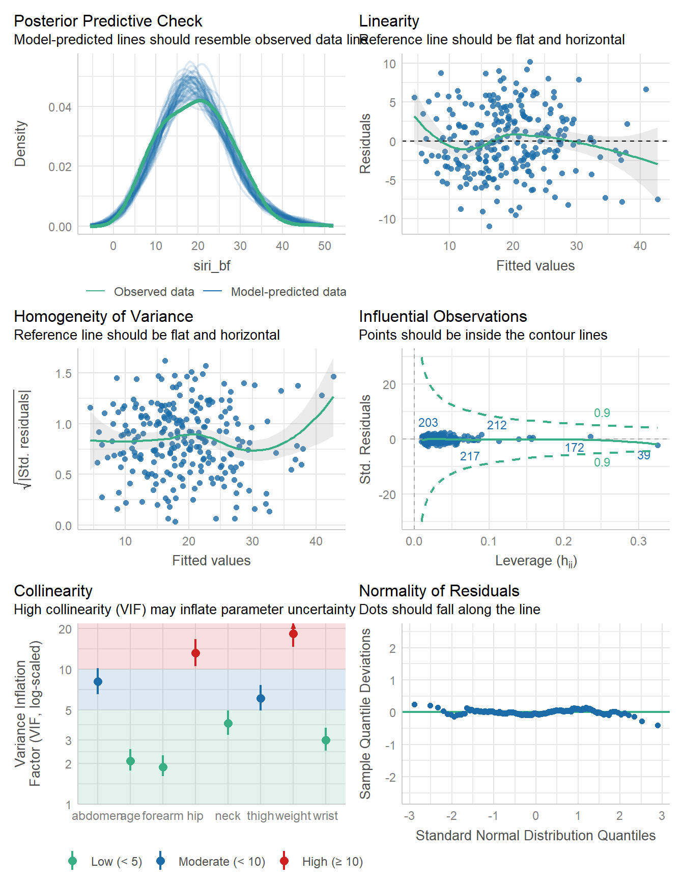
There is still some substantial collinearity here.
19.5.1 Assessing Within-Sample Performance
model_performance(fit2)# Indices of model performance
AIC | AICc | BIC | R2 | R2 (adj.) | RMSE | Sigma
------------------------------------------------------------
1431.9 | 1432.9 | 1467.1 | 0.740 | 0.732 | 4.169 | 4.247compare_performance(fit1, fit2)# Comparison of Model Performance Indices
Name | Model | AIC (weights) | AICc (weights) | BIC (weights) | R2
-----------------------------------------------------------------------
fit1 | lm | 1440.0 (0.017) | 1442.1 (0.010) | 1492.7 (<.001) | 0.742
fit2 | lm | 1431.9 (0.983) | 1432.9 (0.990) | 1467.1 (>.999) | 0.740
Name | R2 (adj.) | RMSE | Sigma
--------------------------------
fit1 | 0.728 | 4.153 | 4.275
fit2 | 0.732 | 4.169 | 4.247plot(compare_performance(fit1, fit2))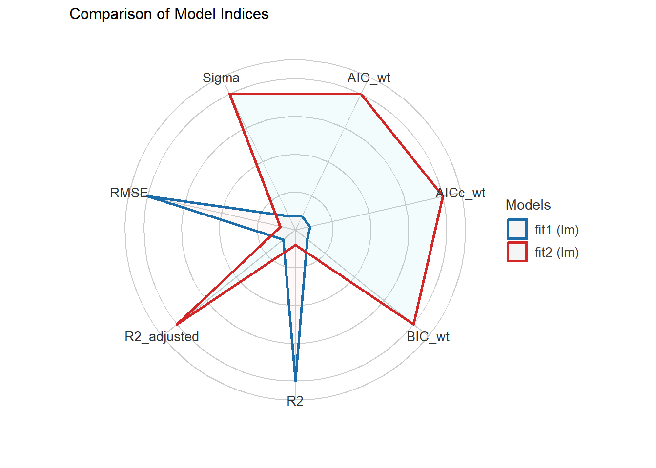
Our \(R^2\) and adjusted \(R^2\) values within the model sample are very similar, as are the AIC and BIC. Other than the raw \(R^2\) (which will always favor the larger model if one is a subset of the predictors in the other) and the root mean squared error, each of these summaries prefers the smaller model fit2.
We can also calculate the mean absolute prediction error (within the data included in our model) with performance_mae() and the root mean squared prediction error (also within our model’s data) with performance_rmse(). Of course, we’ve seen the root mean squared error in the compare_performance() and model_performance() results, already.
performance_mae(fit1)[1] 3.418899performance_mae(fit2)[1] 3.412077performance_rmse(fit1)[1] 4.15292performance_rmse(fit2)[1] 4.16910219.5.2 Using Cross-Validation to assess performance
Next, we’ll use the performance_accuracy() function to estimate the predictive accuracy of our model, using 5-fold cross validation. Note that we set a random seed each time we run this assessment.
- For a linear model, the predictive accuracy measure used is the Pearson correlation \(r\) comparing our model’s predicted values of
siri_bfto the actual observed values. - The output below shows the point estimate of this correlation and a confidence interval around it.
- For some reason, the
easystatspackage shows these correlations as percentages, even though they are not percentages of anything. To obtain estimated \(R^2\) values in our cross-validated sample, we need to express the correlations shown below properly on a scale from 0 to 1, and then square them. - Here we use 5-fold cross-validation (
method = "cv", k = 5) to create our estimates. The data are split by the machine into k (here 5) groups, where the model is refit using 4 of the 5 groups, and then assessed across the fifth group. This is then repeated across all choices of the five groups. The five results are then averaged to obtain the output provided. A bootstrapping approach (withmethod = "boot") is also available for developing these estimates, withinperformance_accuracy().
set.seed(431)
performance_accuracy(fit1, method = "cv",
                     k = 5, ci = 0.95)
# Accuracy of Model Predictions
Accuracy (95% CI): 81.49% [73.12%, 92.09%]
Method: Correlation between observed and predictedset.seed(431)
performance_accuracy(fit2, method = "cv",
k = 5, ci = 0.95)# Accuracy of Model Predictions
Accuracy (95% CI): 82.87% [74.24%, 93.11%]
Method: Correlation between observed and predictedSince we might want to see more than just the correlation coefficient estimated in our cross-validation, we’ll use the performance_cv() function to estimate both RMSE and \(R^2\) for these models.
set.seed(431)
performance_cv(fit1, method = "k_fold", k = 5)
# Cross-validation performance (5-fold method)
MSE | RMSE | R2
-----------------
22 | 4.7 | 0.67set.seed(431)
performance_cv(fit2, method = "k_fold", k = 5)# Cross-validation performance (5-fold method)
MSE | RMSE | R2
----------------
20 | 4.5 | 0.7The performance of the smaller fit2 model looks a little better in these results for both summaries.
19.6 Best Subsets Regression and Mallows’ \(C_p\)
Next, we’ll apply a best subsets regression approach to identify some smaller candidate models.
Here, I’m using ols_step_best_subset() from the olsrr package, which I can use to identify models with high values of \(R^2\) or with low (good) values of such summaries as Mean Squared Error, Mallow’s Cp statistic, or the Akaike Information Criterion. Here, we’ll look at Mallow’s Cp, and consider models which use up to 8 of our candidate predictors.
k <- ols_step_best_subset(fit1,
                          max_order = 8,
                          metric = "cp")
k Best Subsets Regression
--------------------------------------------------------------
Model Index Predictors
--------------------------------------------------------------
1 abdomen
2 weight abdomen
3 weight abdomen wrist
4 weight abdomen forearm wrist
5 weight neck abdomen forearm wrist
6 weight neck abdomen biceps forearm wrist
7 age weight neck abdomen thigh forearm wrist
8 age weight neck abdomen hip thigh forearm wrist
--------------------------------------------------------------
Subsets Regression Summary
--------------------------------------------------------------------------------------------------------------------------------------
Adj. Pred
Model R-Square R-Square R-Square C(p) AIC SBIC SBC MSEP FPE HSP APC
--------------------------------------------------------------------------------------------------------------------------------------
1 0.6543 0.6529 0.6438 69.8409 1488.8082 784.0875 1499.3485 5783.2127 23.5075 0.0952 0.3513
2 0.7143 0.7120 0.7047 17.3601 1443.5224 739.4622 1457.5761 4798.8699 19.5840 0.0793 0.2927
3 0.7233 0.7199 0.7104 11.1761 1437.5707 733.6757 1455.1379 4666.5692 19.1197 0.0774 0.2857
4 0.7304 0.7259 0.7159 6.8132 1433.2074 729.5437 1454.2879 4567.1491 18.7863 0.0761 0.2807
5 0.7335 0.7280 0.7175 5.9241 1432.2633 728.7699 1456.8573 4531.9786 18.7150 0.0758 0.2797
6 0.7355 0.7290 0.7176 6.1051 1432.3916 729.0562 1460.4990 4516.6449 18.7247 0.0759 0.2798
7 0.7378 0.7302 0.7175 6.0319 1432.2408 729.1139 1463.8617 4496.3797 18.7135 0.0759 0.2797
8 0.7403 0.7316 0.7186 5.8272 1431.9331 729.0634 1467.0674 4473.4501 18.6905 0.0758 0.2793
--------------------------------------------------------------------------------------------------------------------------------------
AIC: Akaike Information Criteria
SBIC: Sawa's Bayesian Information Criteria
SBC: Schwarz Bayesian Criteria
MSEP: Estimated error of prediction, assuming multivariate normality
FPE: Final Prediction Error
HSP: Hocking's Sp
APC: Amemiya Prediction Criteria plot(k)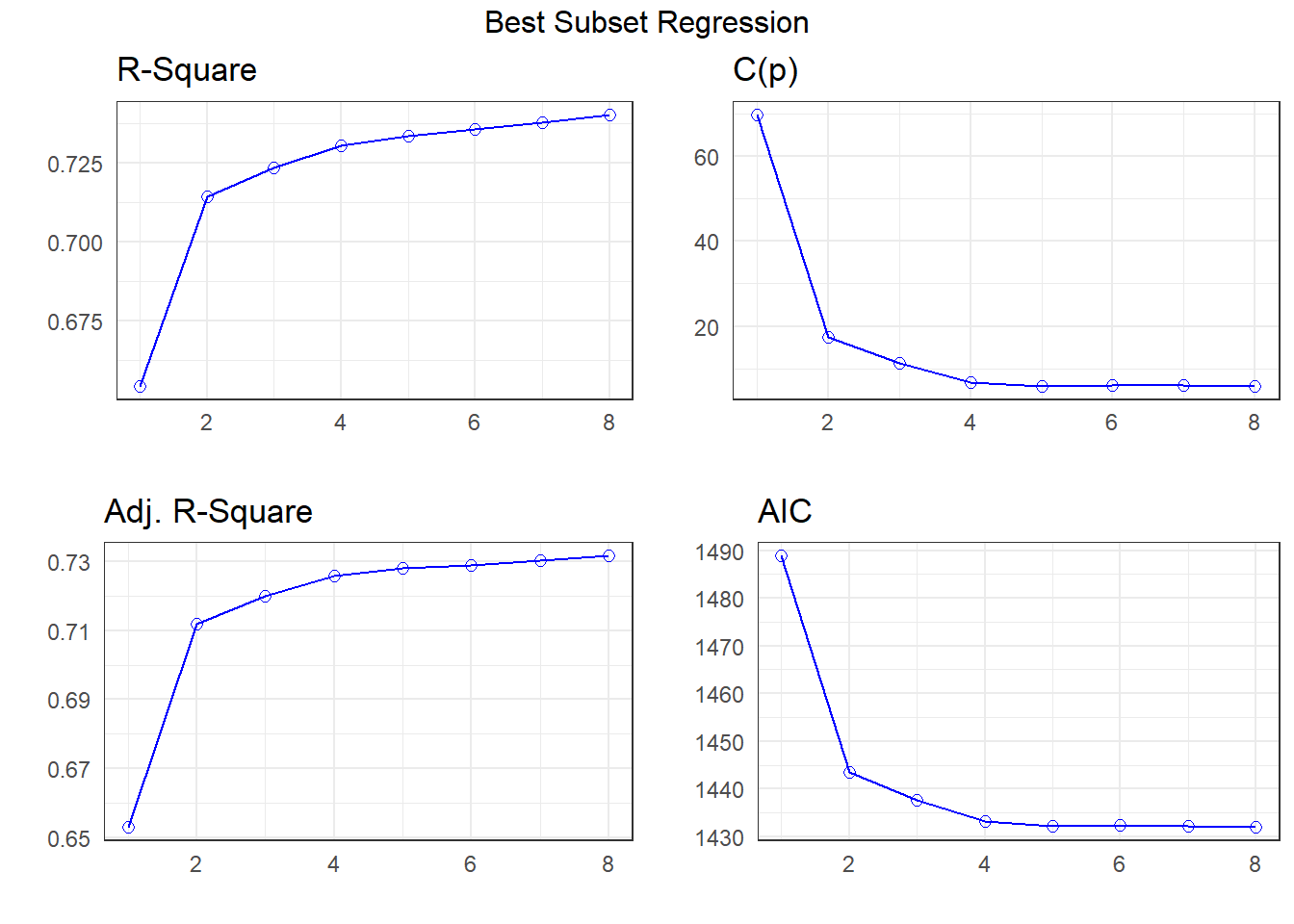
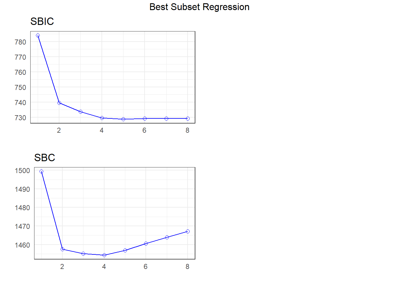
Looking at the Cp plot, I see that most of the progress down has happened at either 4 or 5 predictors, so I’ll consider those models.
19.7 Four-Predictor Model
Here is the four-predictor model from our Best Subsets Regression output.
fit4 <- lm(
  siri_bf ~ weight + abdomen + forearm + wrist,
  data = bodyfat
) model_parameters(fit4, ci = 0.95)Parameter | Coefficient | SE | 95% CI | t(243) | p
---------------------------------------------------------------------
(Intercept) | -33.61 | 7.26 | [-47.91, -19.32] | -4.63 | < .001
weight | -0.14 | 0.02 | [ -0.19, -0.09] | -5.58 | < .001
abdomen | 0.99 | 0.06 | [ 0.88, 1.10] | 17.71 | < .001
forearm | 0.45 | 0.18 | [ 0.10, 0.81] | 2.51 | 0.013
wrist | -1.48 | 0.44 | [ -2.36, -0.61] | -3.34 | < .001
Uncertainty intervals (equal-tailed) and p-values (two-tailed) computed
using a Wald t-distribution approximation.model_performance(fit4)# Indices of model performance
AIC | AICc | BIC | R2 | R2 (adj.) | RMSE | Sigma
------------------------------------------------------------
1433.2 | 1433.6 | 1454.3 | 0.730 | 0.726 | 4.248 | 4.291The \(R^2\) here indicates that about 73% of the variation in siri_bf in the data used for modeling has been explained by fit4. Note that this is quite close to where we started. How do regression assumptions look?
check_model(fit4)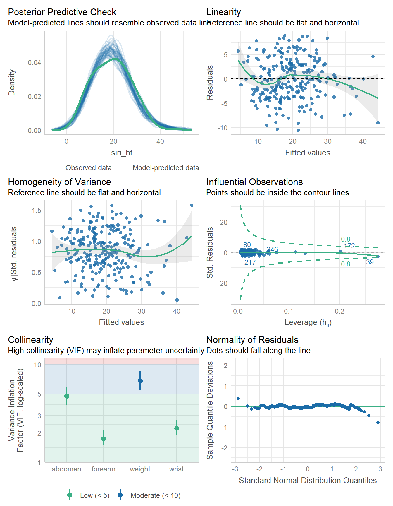
These diagnostic plots look pretty good. We have less troubling collinearity, for one thing, although the distribution from our model still doesn’t quite match the observed data.
19.8 Five-Predictor Model
Now, here is the five-predictor model from our Best Subsets Regression output.
fit5 <- lm(
  siri_bf ~ weight + neck + abdomen + forearm + wrist,
  data = bodyfat
)model_parameters(fit5, ci = 0.95)Parameter | Coefficient | SE | 95% CI | t(242) | p
---------------------------------------------------------------------
(Intercept) | -29.23 | 7.67 | [-44.35, -14.11] | -3.81 | < .001
weight | -0.12 | 0.03 | [ -0.17, -0.07] | -4.81 | < .001
neck | -0.37 | 0.22 | [ -0.81, 0.06] | -1.70 | 0.090
abdomen | 1.00 | 0.06 | [ 0.89, 1.11] | 17.85 | < .001
forearm | 0.51 | 0.18 | [ 0.15, 0.87] | 2.79 | 0.006
wrist | -1.23 | 0.47 | [ -2.15, -0.31] | -2.62 | 0.009
Uncertainty intervals (equal-tailed) and p-values (two-tailed) computed
using a Wald t-distribution approximation.model_performance(fit5)# Indices of model performance
AIC | AICc | BIC | R2 | R2 (adj.) | RMSE | Sigma
------------------------------------------------------------
1432.3 | 1432.7 | 1456.9 | 0.734 | 0.728 | 4.223 | 4.275check_model(fit5)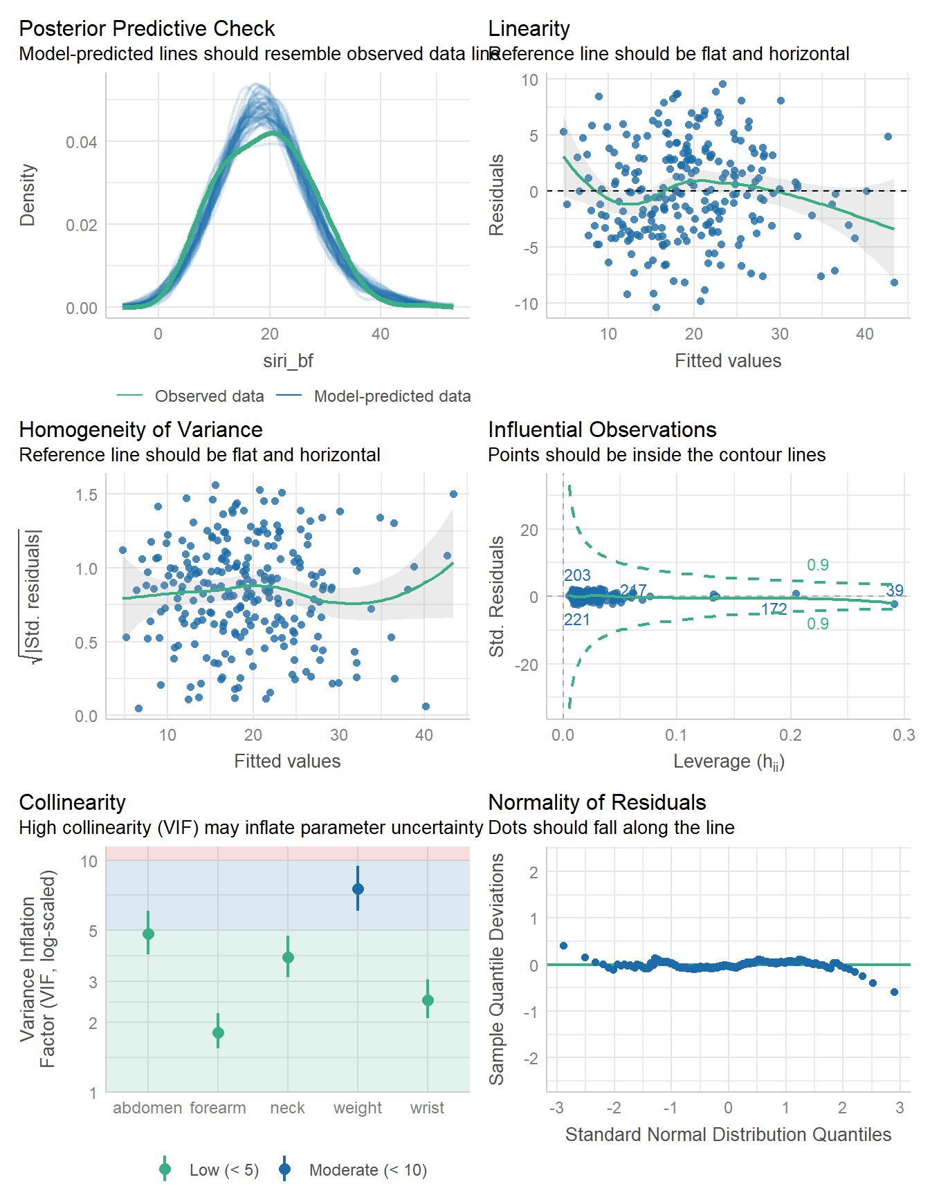
compare_performance(fit4, fit5)# Comparison of Model Performance Indices
Name | Model | AIC (weights) | AICc (weights) | BIC (weights) | R2
-----------------------------------------------------------------------
fit4 | lm | 1433.2 (0.384) | 1433.6 (0.398) | 1454.3 (0.783) | 0.730
fit5 | lm | 1432.3 (0.616) | 1432.7 (0.602) | 1456.9 (0.217) | 0.734
Name | R2 (adj.) | RMSE | Sigma
--------------------------------
fit4 | 0.726 | 4.248 | 4.291
fit5 | 0.728 | 4.223 | 4.275set.seed(431)
performance_accuracy(fit1, method = "cv", k = 5)# Accuracy of Model Predictions
Accuracy (95% CI): 81.49% [73.12%, 92.09%]
Method: Correlation between observed and predictedset.seed(431)
performance_accuracy(fit2, method = "cv", k = 5)# Accuracy of Model Predictions
Accuracy (95% CI): 82.87% [74.24%, 93.11%]
Method: Correlation between observed and predictedset.seed(431)
performance_accuracy(fit4, method = "cv", k = 5)# Accuracy of Model Predictions
Accuracy (95% CI): 83.10% [74.74%, 92.71%]
Method: Correlation between observed and predictedset.seed(431)
performance_accuracy(fit5, method = "cv", k = 5)# Accuracy of Model Predictions
Accuracy (95% CI): 82.99% [74.96%, 93.04%]
Method: Correlation between observed and predictedset.seed(431)
performance_cv(fit1)# Cross-validation performance (30% holdout method)
MSE | RMSE | R2
-----------------
16 | 4 | 0.74set.seed(431)
performance_cv(fit2)# Cross-validation performance (30% holdout method)
MSE | RMSE | R2
-----------------
15 | 3.8 | 0.76set.seed(431)
performance_cv(fit4)# Cross-validation performance (30% holdout method)
MSE | RMSE | R2
-----------------
14 | 3.8 | 0.76set.seed(431)
performance_cv(fit5)# Cross-validation performance (30% holdout method)
MSE | RMSE | R2
-----------------
15 | 3.9 | 0.75Overall, I don’t see a lot here that suggests using fit5 instead of fit4. The diagnostic plots are similar in their successes and failures, and the cross-validated performance looks a little better with fit4.
19.9 Bayesian linear model
For completeness, we’ll now refit the four-predictor model using stan_glm() and a weakly informative prior, as usual.
fit4b <- stan_glm(
  siri_bf ~ weight + abdomen + forearm + wrist,
  data = bodyfat, refresh = 0
) model_parameters(fit4b, ci = 0.95)Parameter | Median | 95% CI | pd | Rhat | ESS | Prior
-----------------------------------------------------------------------------------------
(Intercept) | -33.40 | [-48.11, -19.22] | 100% | 1.003 | 2889 | Normal (19.28 +- 20.49)
weight | -0.14 | [ -0.19, -0.09] | 100% | 1.004 | 2119 | Normal (0.00 +- 0.71)
abdomen | 0.99 | [ 0.87, 1.10] | 100% | 1.002 | 2402 | Normal (0.00 +- 1.92)
forearm | 0.45 | [ 0.09, 0.81] | 99.40% | 1.001 | 3820 | Normal (0.00 +- 10.20)
wrist | -1.49 | [ -2.35, -0.59] | 99.95% | 1.002 | 3160 | Normal (0.00 +- 22.30)
Uncertainty intervals (equal-tailed) computed using a MCMC distribution
approximation.model_performance(fit4b)# Indices of model performance
ELPD | ELPD_SE | LOOIC | LOOIC_SE | WAIC | R2 | R2 (adj.) | RMSE | Sigma
-----------------------------------------------------------------------------------
-717.391 | 9.727 | 1434.8 | 19.455 | 1434.6 | 0.727 | 0.716 | 4.248 | 4.300check_model(fit4b)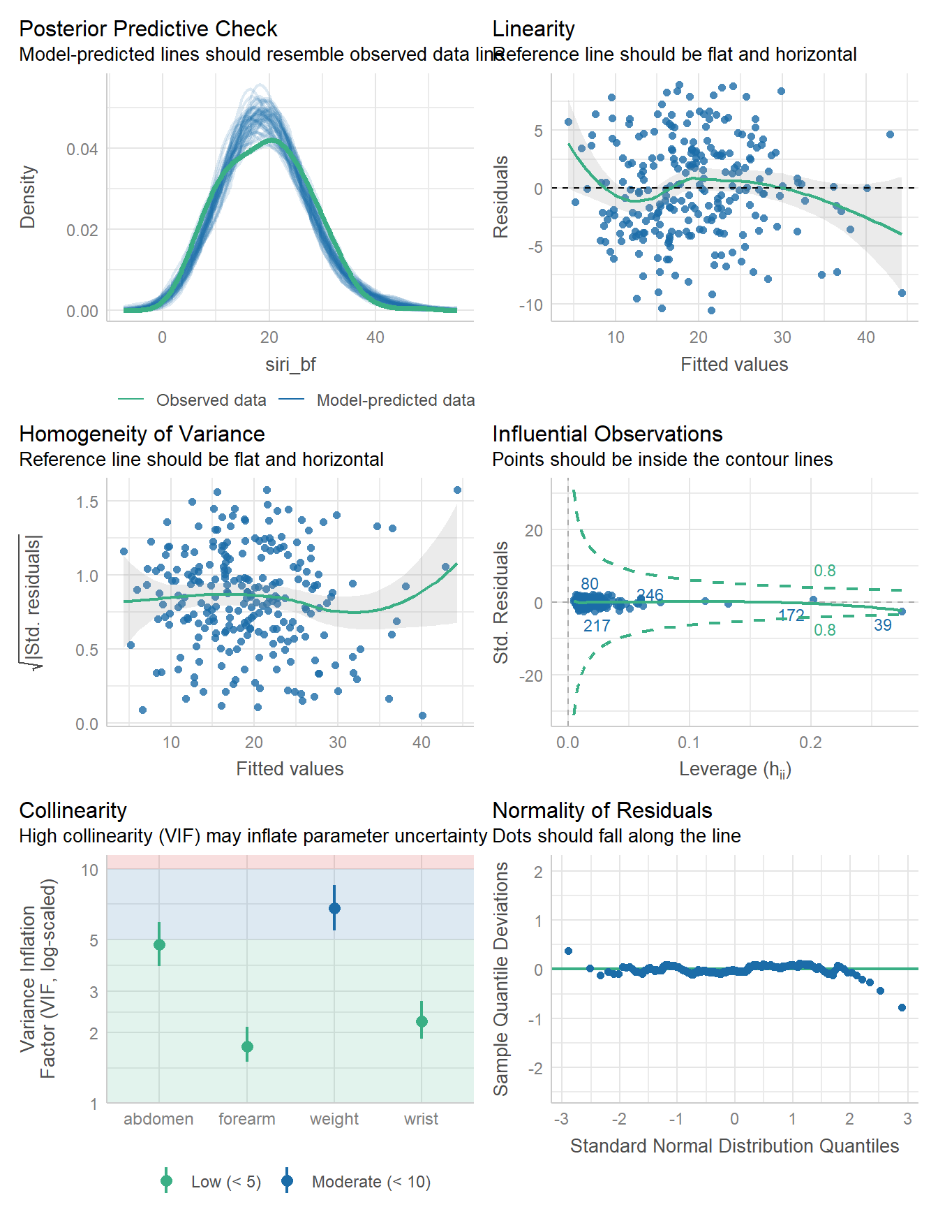
set.seed(431)
performance_accuracy(fit4b, method = "cv", k = 5)
# Accuracy of Model Predictions
Accuracy (95% CI): 83.11% [74.77%, 92.71%]
Method: Correlation between observed and predictedset.seed(431)
performance_cv(fit4b)# Cross-validation performance (30% holdout method)
MSE | RMSE | R2
-----------------
14 | 3.8 | 0.76Again, these results look very similar to fit4.
19.10 For More Information
- The easystats packages have lots of tools we’ve seen here, including
compare_performance(),performance_mae(),performance_accuracy(), andperformance_cv(). - Wikipedia on Cross-validation is pretty useful.
- Model selection is an especially bad idea in building clinical prediction models, as it turns out. Frank Harrell (Harrell 2015) has much more on this subject.
- Stepwise model selection, overall, is pretty terrible. See, for instance, this blog post “Stepwise selection of variables in regression is Evil” from Free range statistics, which concludes…
That’s all folks. Just don’t use stepwise selection of variables. Don’t use automated addition and deletion of variables, and don’t take them out yourself by hand “because it’s not significant”. Use theory-driven model selection if it’s explanation you’re after, Bayesian methods are going to be good too as a complement to that and forcing you to think about the problem; and for regression-based prediction use a lasso or elastic net regularization.
We’ll talk about the LASSO and elastic net in 432. 3.