17 Two Factor ANOVA
17.1 R setup for this chapter
Appendix A lists all R packages used in this book, and also provides R session information. Appendix B describes the 431-Love.R script, and demonstrates its use.
17.2 Data are Rosner’s FEV Data
Appendix C provides further guidance on pulling data from other systems into R, while Appendix D gives more information (including download links) for all data sets used in this book.
Rosner’s FEV data, found at (for instance) https://hbiostat.org/data/ includes information on forced expiratory volume, abbreviated FEV (quant) as a function of several covariates. The data are also available to you on our 431-data site as fev_ros.csv.
fev_ros <- read_csv("data/fev_ros.csv", show_col_types = FALSE) |>
  mutate(across(where(is.character), as_factor)) |>
  mutate(id = as.character(id))

fev_ros
# A tibble: 654 × 6
id age fev height sex smoke
<chr> <dbl> <dbl> <dbl> <fct> <fct>
1 301 9 1.71 57 female non-current smoker
2 451 8 1.72 67.5 female non-current smoker
3 501 7 1.72 54.5 female non-current smoker
4 642 9 1.56 53 male non-current smoker
5 901 9 1.90 57 male non-current smoker
6 1701 8 2.34 61 female non-current smoker
7 1752 6 1.92 58 female non-current smoker
8 1753 6 1.42 56 female non-current smoker
9 1901 8 1.99 58.5 female non-current smoker
10 1951 9 1.94 60 female non-current smoker
# ℹ 644 more rowsn_miss(fev_ros)[1] 0Our primary interest here is in estimating how fev, a quantitative outcome, varies by the two levels of sex (male or female) and the two levels of smoke (current smoker or non-current) available in the data.
We should begin with an interaction plot as a way of summarizing these relationships.
17.3 Interaction Plot
17.3.1 Simple Plot of Means
fev_ros |> group_by(sex, smoke) |>
  summarise(mean_fev = mean(fev)) |>
  ggplot(aes(x = sex, y = mean_fev, group = smoke, col = smoke)) +
  geom_point() +
  geom_line() +
  scale_color_metro_d() +
  labs(x = "sex", y = "Mean of FEV")
`summarise()` has grouped output by 'sex'. You can override using the `.groups`
argument.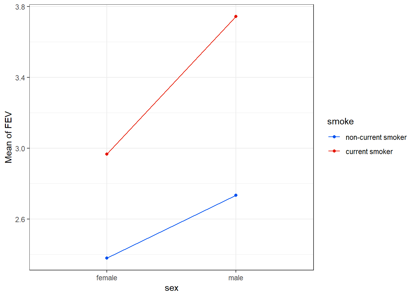
Let’s add labels to show the values of the mean within each of the four groups formed by the combinations of two sex levels and two smoke levels.
17.3.2 Labeled Interaction Plot
fev_ros |> group_by(sex, smoke) |>
  summarise(mean_fev = mean(fev)) |>
  ggplot(aes(x = smoke, y = mean_fev, group = sex, col = sex)) +
  geom_line() +
  geom_label(aes(label = round(mean_fev,2))) +
  scale_color_see_d() +
  labs(x = "Smoking Status", y = "Mean of FEV",
       title = "Interaction of Sex and Smoking Status on Mean of FEV",
       subtitle = "Rosner data")
`summarise()` has grouped output by 'sex'. You can override using the `.groups`
argument.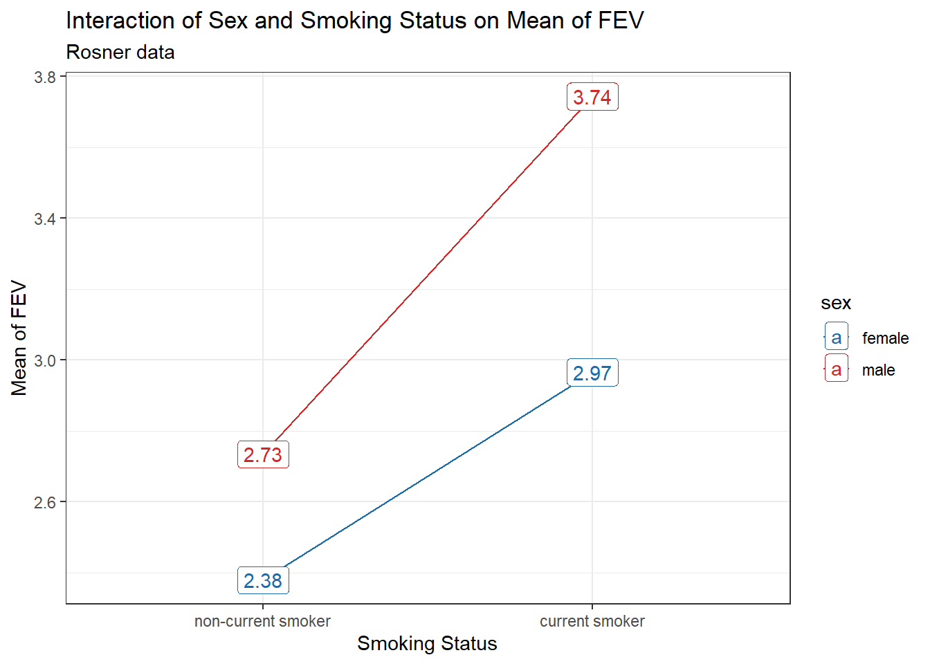
An important purpose of this plot is to show us whether or not it seems likely that an interaction term will be required in our model. We observe somewhat non-parallel lines here, where the difference between males and females is a bit smaller for non-current smokers than it is for current smokers. This suggests we consider including an interaction in our model. So let’s try that.
17.4 ANOVA models
The model fit1 is a two-way analysis of variance model predicting fev using sex, smoke, and the interaction of sex and smoke.
fit1 <- aov(fev ~ sex * smoke, data = fev_ros)

model_parameters(fit1, es_type = "eta", ci = 0.95)
Parameter | Sum_Squares | df | Mean_Square | F | p | Eta2 (partial) | Eta2 95% CI
--------------------------------------------------------------------------------------------
sex | 21.32 | 1 | 21.32 | 31.98 | < .001 | 0.05 | [0.02, 1.00]
smoke | 33.68 | 1 | 33.68 | 50.51 | < .001 | 0.07 | [0.04, 1.00]
sex:smoke | 2.51 | 1 | 2.51 | 3.77 | 0.053 | 5.76e-03 | [0.00, 1.00]
Residuals | 433.40 | 650 | 0.67 | | | |
Anova Table (Type 1 tests)We can see from the sums of squares that the sex by smoke interaction only accounts about 4.4% of the variation explained by the model1, and less than 1% of the variation in fev overall2
Since this ANOVA model is just a linear regression model, the model fit2 below, which includes the same predictors, is in fact the same model as fit1.
fit2 <- lm(fev ~ sex * smoke, data = fev_ros)

model_parameters(fit2, ci = 0.95)
Parameter | Coefficient | SE | 95% CI
------------------------------------------------------------------------
(Intercept) | 2.38 | 0.05 | [ 2.28, 2.48]
sex [male] | 0.36 | 0.07 | [ 0.22, 0.49]
smoke [current smoker] | 0.59 | 0.14 | [ 0.31, 0.86]
sex [male] × smoke [current smoker] | 0.42 | 0.22 | [ 0.00, 0.85]
Parameter | t(650) | p
-----------------------------------------------------
(Intercept) | 48.67 | < .001
sex [male] | 5.27 | < .001
smoke [current smoker] | 4.20 | < .001
sex [male] × smoke [current smoker] | 1.94 | 0.053
Uncertainty intervals (equal-tailed) and p-values (two-tailed) computed
  using a Wald t-distribution approximation.
17.4.1 Bootstrapping CIs for estimates
set.seed(431)
model_parameters(fit2,
           ci = 0.95, ci_method = "quantile",
           bootstrap = TRUE, iteractions = 1000)
Parameter | Coefficient | 95% CI | p
--------------------------------------------------------------------------
(Intercept) | 2.38 | [ 2.31, 2.45] | < .001
sex [male] | 0.35 | [ 0.22, 0.49] | < .001
smoke [current smoker] | 0.58 | [ 0.44, 0.73] | < .001
sex [male] × smoke [current smoker] | 0.43 | [-0.01, 0.81] | 0.052
Uncertainty intervals (equal-tailed) are naıve bootstrap intervals.The bootstrap confidence interval for the interaction term confirms our findings from the ANOVA and the linear model that the interaction effect could be very small. Suppose we instead consider the model including just the main effects of the factors sex and smoke, as in fit3 below.
17.5 ANOVA without interaction
fit3 <- aov(fev ~ sex + smoke, data = fev_ros)

model_parameters(fit3, es_type = "eta", ci = 0.95)
Parameter | Sum_Squares | df | Mean_Square | F | p | Eta2 (partial) | Eta2 95% CI
--------------------------------------------------------------------------------------------
sex | 21.32 | 1 | 21.32 | 31.85 | < .001 | 0.05 | [0.02, 1.00]
smoke | 33.68 | 1 | 33.68 | 50.30 | < .001 | 0.07 | [0.04, 1.00]
Residuals | 435.91 | 651 | 0.67 | | | |
Anova Table (Type 1 tests)We can compare the results from our model without interaction (fit3) and the model with interaction (fit1) using an F test, as follows.
anova(fit3, fit1)Analysis of Variance Table
Model 1: fev ~ sex + smoke
Model 2: fev ~ sex * smoke
Res.Df RSS Df Sum of Sq F Pr(>F)
1 651 435.91
2 650 433.40 1 2.5127 3.7684 0.05266 .
---
Signif. codes: 0 '***' 0.001 '**' 0.01 '*' 0.05 '.' 0.1 ' ' 1Again, we don’t have strong evidence of a substantial interaction effect here.
17.6 Considering Model Diagnostics
Let’s consider the regression model diagnostics for our two candidate models.
check_model(fit1)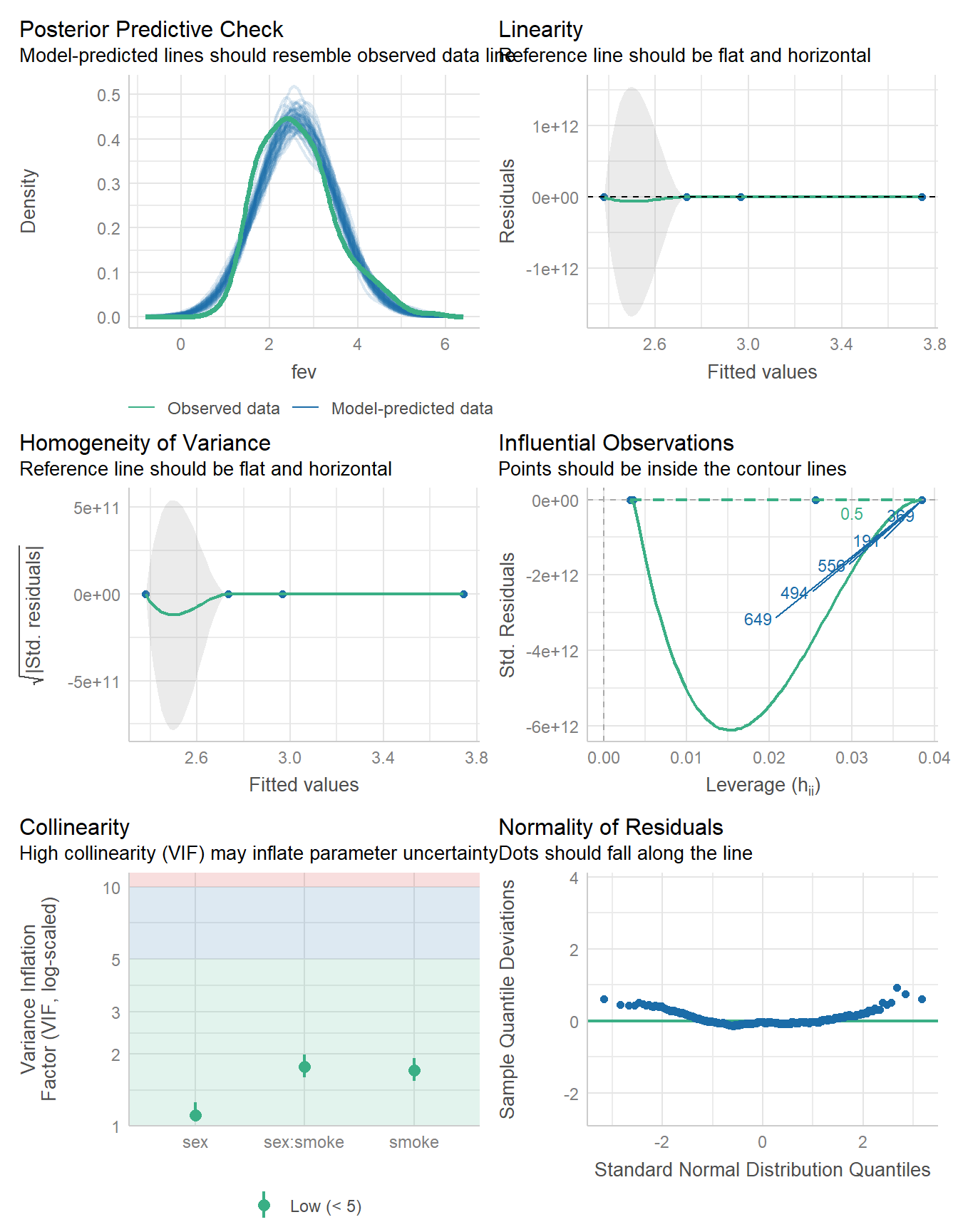
check_model(fit3)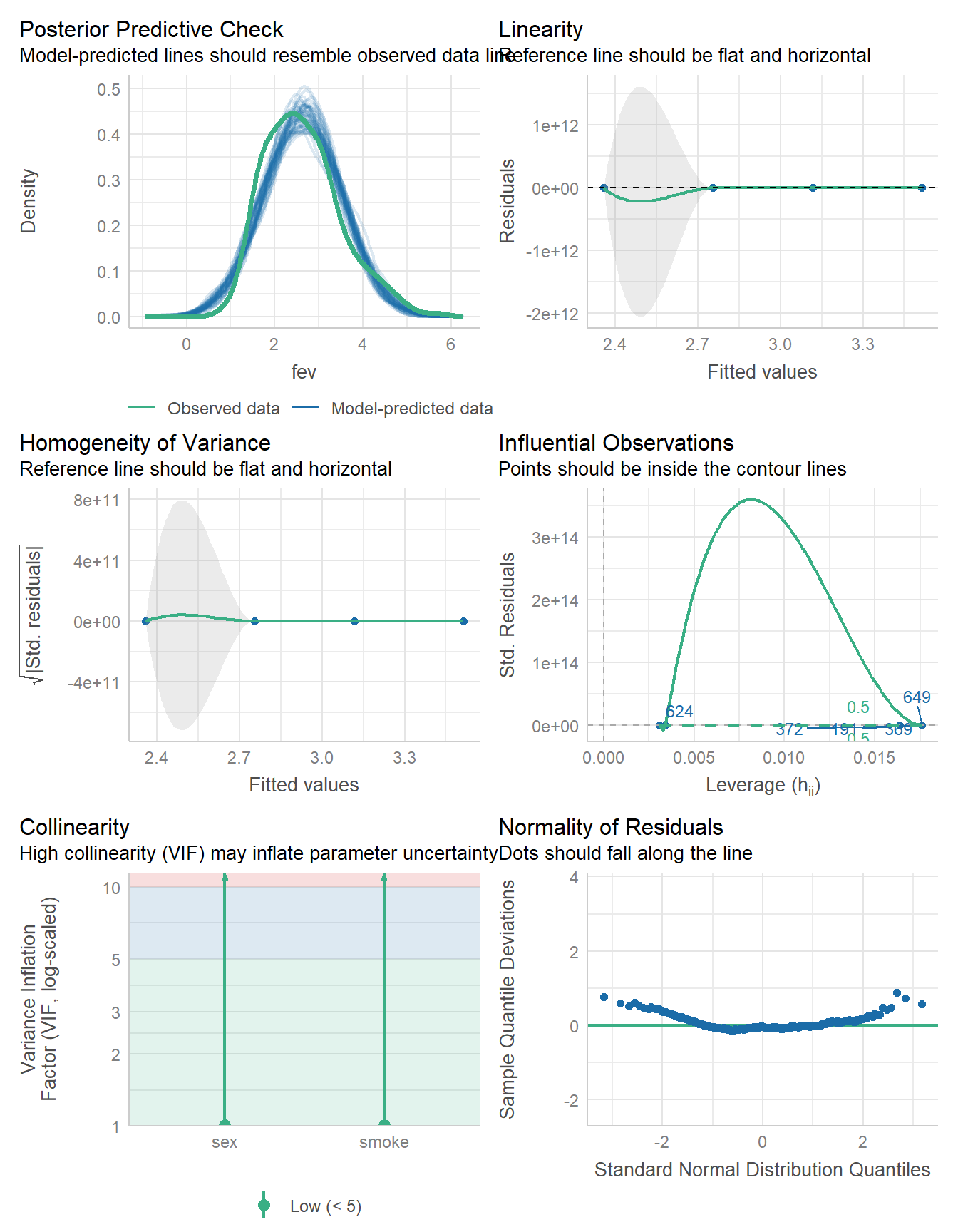
The models look fairly similar in terms of these diagnostic plots. So far, I am inclined to use the model without interaction. We can also compare their performance on various summary statistics.
17.7 Comparing Model Performance
compare_performance(fit1, fit3)# Comparison of Model Performance Indices
Name | Model | AIC (weights) | AICc (weights) | BIC (weights) | R2
-----------------------------------------------------------------------
fit1 | aov | 1596.9 (0.709) | 1597.0 (0.706) | 1619.3 (0.206) | 0.117
fit3 | aov | 1598.7 (0.291) | 1598.7 (0.294) | 1616.6 (0.794) | 0.112
Name | R2 (adj.) | RMSE | Sigma
--------------------------------
fit1 | 0.113 | 0.814 | 0.817
fit3 | 0.109 | 0.816 | 0.818plot(compare_performance(fit1, fit3))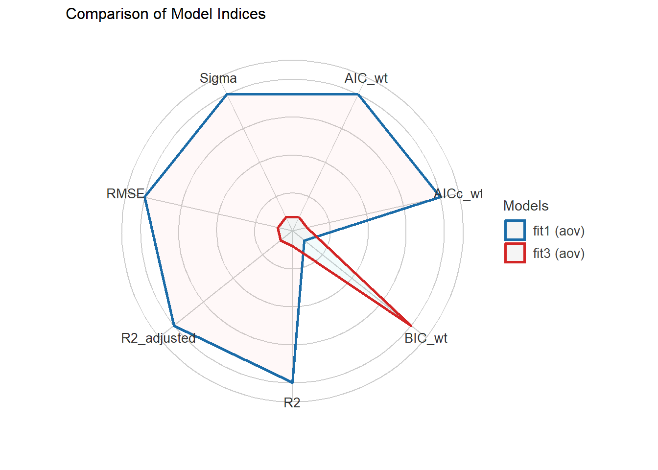
On these measures of model performance, our fit1 model outperforms the model without interaction on every measure except for BIC, although the differences are very small in each case (for example, \(R^2\) is 0.117 with the interaction and 0.113 without.)
Making a final decision between these models (assuming no test data are available) would likely come down to:
- whether the interaction’s estimated effect seems large enough to be important,
- whether the investigator interprets the diagnostic plots as strongly favoring either model over the other,
- whether the clinical/scientific information we have prior to completing the study (as the result of logic, theory and empirical evidence) is strongly suggestive that an interaction term should or should not be included in the final model.
Given no other information, I would probably go with the smaller model (fit3) here, but you could certainly make a case either way.
17.8 For More Information
- Understanding Two-Way Interactions at https://library.virginia.edu/data/articles/understanding-2-way-interactions is a useful summary from the University of Virginia Library’s Research Data Services group.
- The Wikipedia page for Two-Way Analysis of Variance provides most of the necessary mathematics, and describes a bit of the history.