5  Comparing Paired Samples

5.1 R setup for this chapter

Note

This section loads all needed R packages for this chapter. Appendix A lists all R packages used in this book, and also provides R session information. Appendix B describes the 431-Love.R script, and demonstrates its use.

library(infer)
library(knitr)
library(naniar)
library(patchwork)
library(rstanarm)

library(easystats)
library(tidyverse)

source("data/Love-431.R")
theme_set(theme_bw())

5.2 Data: Lead in the Blood of Children

Note

Appendix C provides further guidance on pulling data from other systems into R, while Appendix D gives more information (including download links) for all data sets used in this book.

Morton et al. (1982) studied the absorption of lead into the blood of children in a matched-sample study. The “exposed” subjects were 33 children whose parents worked in a battery manufacturing factory (where lead was used) in Oklahoma. Each child with a lead-exposed parent was then matched to another child of the same age with similar exposure to traffic who lived in the same neighborhood, but whose parents did not work in lead-related industries.

The complete study thus contains 66 children, arranged into 33 matched pairs. A sample of whole blood from each child provides the outcome of interest, which is lead content, measured in mg/dl.

Mainly, we want to estimate the difference in lead content between the exposed and control children, and then use that sample estimate to make inferences about the difference in lead content between the population of all children like those in the exposed group and the population of all children like those in the control group.

The data are available in several places, including the PairedData package in R and Pruzek and Helmreich (2009), but here we ingest the bloodlead.csv file from our website. A table of the first few pairs of observations (blood lead levels for one child exposed to lead and the matched control) is shown below.

bloodlead <- read_csv("data/bloodlead.csv", show_col_types = FALSE)

bloodlead

# A tibble: 33 × 3
   pair  exposed control
   <chr>   <dbl>   <dbl>
 1 P01        38      16
 2 P02        23      18
 3 P03        41      18
 4 P04        18      24
 5 P05        37      19
 6 P06        36      11
 7 P07        23      10
 8 P08        62      15
 9 P09        31      16
10 P10        34      18
# ℹ 23 more rows

So, for instance, the first pair includes an exposed child whose blood lead level was 38 mg/dl and an unexposed (control) child whose blood lead level was 16 mg/dl. Using the n_miss() function from the naniar package, we see complete data in all 33 rows.

n_miss(bloodlead)

[1] 0

5.3 Paired Differences

Since we are interested in comparing the differences between the exposed and control children, we first create a column of these paired differences.

bloodlead <- bloodlead |>
  mutate(difference = exposed - control)

bloodlead |> head()

# A tibble: 6 × 4
  pair  exposed control difference
  <chr>   <dbl>   <dbl>      <dbl>
1 P01        38      16         22
2 P02        23      18          5
3 P03        41      18         23
4 P04        18      24         -6
5 P05        37      19         18
6 P06        36      11         25

Again, the first pair includes an exposed child with blood lead level of 38 mg/dl and an unexposed (control) child measured at 16 mg/dl. So that paired difference is 38 - 16 = 22 mg/dl.

5.3.1 Visualizing the sample

To help our understanding of the distribution of our paired differences, we might, for instance, prepare a histogram, a boxplot (with violin) or a Normal Q-Q plot. Below, we show all three summaries, using the patchwork package to bind together the three individual ggplot2 plots.

bw <- 8 # specify width of bins in histogram

p1 <- ggplot(bloodlead, aes(difference)) +
  geom_histogram(binwidth = bw, fill = "black", col = "yellow" ) +
  stat_function(fun = function(x) {
    dnorm(x, mean = mean(bloodlead$difference, na.rm = TRUE),
          sd = sd(bloodlead$difference, na.rm = TRUE) ) *
        length(bloodlead$difference) * bw},
    geom = "area", alpha = 0.5, fill = "lightblue", col = "blue") +
  labs(x = "Exposed - Control lead (mg/dl)",
    title = "Histogram & Normal Curve")

p2 <- ggplot(bloodlead, aes(sample = difference)) +
  geom_qq() +
  geom_qq_line(col = "red") +
  labs(y = "Exposed - Control", x = "Standard Normal Distribution",
    title = "Normal Q-Q plot")

p3 <- ggplot(bloodlead, aes(x = difference, y = "")) +
  geom_violin(fill = "cornsilk") +
  geom_boxplot(width = 0.2) +
  stat_summary(fun = mean, geom = "point", shape = 16, col = "red") +
  labs(y = "", x = "Exposed - Control", title = "Boxplot with Violin")

p1 + (p2 / p3 + plot_layout(heights = c(2, 1))) +
  plot_annotation(title = "Exposed - Control Differences in Blood Lead Content, mg/dl")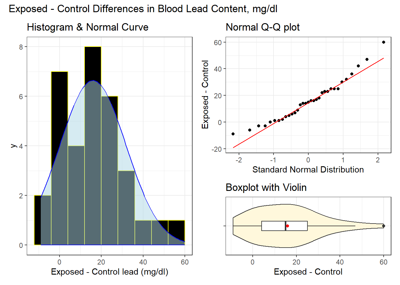

The center of the distribution appears to be around 15 mg/dl according to these plots. The data range from below 0 (around -10) to 60 mg/dl. In terms of shape, each of these plots seems to suggest an approximately Normal distribution. There’s a single candidate outlier out to the right of the distribution (at 60 mg/dl), but that doesn’t seem to be a major concern at this stage.

5.3.2 Numerical Summaries

Here are a few of the more useful numerical summaries we might consider in developing our understanding of the paired Exposed - Control differences in blood lead levels.

bloodlead |>
  reframe(lovedist(difference)) |>
  kable(digits = 2)

n	miss	mean	sd	med	mad	min	q25	q75	max
33	0	15.97	15.86	15	14.83	-9	4	25	60

Across these 33 paired differences, the mean and median are within one mg/dl of each other. The standard deviation is near 16 mg/dl and the mad just a bit less than 15 mg/dl. The quartiles match our expectations from the plots.

5.4 Estimating the Mean Difference

Next, we will provide a point estimate and confidence interval for the average difference. Of course, we might consider the average to be the mean or the median (or even something else.) To start, we’ll focus on obtaining an estimate and sense of uncertainty around that estimate for the mean of the paired differences.

We saw previously that the sample mean of those 33 differences is about 16 mg/dl, and that the distribution of those paired differences in blood lead content are approximately Normally distributed. In light of those findings, how can we put an interval around that estimate that expresses our uncertainty in a reasonable way?

5.4.1 Using a linear model

The most general approach is to fit a linear model to the data. When working with one sample, like these paired differences contained in the difference column in the bloodlead tibble, we will start by running this model:

fit1 <- lm(difference ~ 1, data = bloodlead)

Here, the use of the number one indicates to R that we wish to fit a model for difference using only an intercept term. What does this model produce?

fit1

Call:
lm(formula = difference ~ 1, data = bloodlead)

Coefficients:
(Intercept)  
      15.97  

The fit here provides an estimate, which turns out to be the sample mean of the paired differences, or 15.97 mg/dl.

To obtain a confidence interval around this estimate, we might consider the confint() function.

confint(fit1, level = 0.95)

               2.5 %  97.5 %
(Intercept) 10.34469 21.5947

This provides a 95% confidence interval for the mean of the paired differences. We might state this combination of results as follows:

• Our sample of 33 pairs of exposed and control children shows an average difference in blood lead levels of 15.97 mg/dl with a 95% confidence interval ranging from (10.34, 21.59) mg/dl.
• Suppose Harry receives the exposure and Ron does not, but in all other ways they are similar, in the same way that our matched pairs were formed. Then our model suggests that Harry’s blood level will be 15.97 mg/dl larger than Ron’s.

Note

We might further describe this point and interval estimate combination as a result from a paired-samples comparison, via an intercept-only linear model. The result we have obtained here, as it turns out, is identical that obtained by building a paired t-test for the mean difference.

What if we instead wanted to see a 90% confidence interval for the mean?

confint(fit1, level = 0.9)

                 5 %     95 %
(Intercept) 11.29201 20.64738

• Now, our sample of 33 pairs of exposed and control children shows an average difference in blood lead levels of 15.97 mg/dl with a 90% confidence interval ranging from (11.29, 20.65) mg/dl.

Note

• Note that the 90% confidence interval is thinner than the 95% confidence interval. Why do you think that is true?

For more details on our linear model, we might use the summary() function in R, as follows:

summary(fit1)

Call:
lm(formula = difference ~ 1, data = bloodlead)

Residuals:
   Min     1Q Median     3Q    Max 
-24.97 -11.97  -0.97   9.03  44.03 

Coefficients:
            Estimate Std. Error t value Pr(>|t|)    
(Intercept)   15.970      2.762   5.783 2.04e-06 ***
---
Signif. codes:  0 '***' 0.001 '**' 0.01 '*' 0.05 '.' 0.1 ' ' 1

Residual standard error: 15.86 on 32 degrees of freedom

Here’s what we find in this summary:

1. A restatement of the fitted model.
2. A five-number summary (minimum, 25th percentile, median, 75th percentile and maximum) of the model residuals (which are the observed - predicted errors made by the model.)
   • So the median of the errors we made in using this model to predict a difference appears to be that our prediction was 0.97 mg/dl too high.
3. Some information about the coefficient of the model, specifically its point estimate (15.97) and its standard error (2.76).
   • Remember we can obtain an approximate 95% confidence interval for this estimate by adding and subtracting two times its standard error.
   • We also see a t statistic, p value (that’s the Pr(>|t|) piece) and some codes related to statistical significance. I’ll ignore all of that, at least until Chapter 15.
4. Finally we see an estimated residual standard error, which is an estimate of an important quality called \(\sigma\), or sigma.

The summary() function after a model is a very common approach in R, and it provides lots of useful information.

However, in this book, we will make heavy use of a few alternative approaches available in the easystats ecosystem of packages, specifically model_parameters() and model_performance(), to obtain and amplify the information we get from summary().

First, let’s look at what model_parameters() provides…

fit1 |>
  model_parameters(ci = 0.95) |>
  kable(digits = 2)

Parameter	Coefficient	SE	CI	CI_low	CI_high	t	df_error	p
(Intercept)	15.97	2.76	0.95	10.34	21.59	5.78	32	0

This adds the 95% confidence interval for our estimate, which remains (10.34, 21.59) rounded to two decimal places.

What if we wanted to see a 90% confidence interval, instead of 95%?

fit1 |>
  model_parameters(ci = 0.9) |>
  kable(digits = 2)

Parameter	Coefficient	SE	CI	CI_low	CI_high	t	df_error	p
(Intercept)	15.97	2.76	0.9	11.29	20.65	5.78	32	0

5.4.2 Using t.test()

The one-sample t-test on the paired differences produces the same confidence interval and other summaries as the paired-samples test comparing the exposed to the control directly, as we see below.

fit2 <- t.test(bloodlead$difference, conf.level = 0.95)

fit2

    One Sample t-test

data:  bloodlead$difference
t = 5.783, df = 32, p-value = 2.036e-06
alternative hypothesis: true mean is not equal to 0
95 percent confidence interval:
 10.34469 21.59470
sample estimates:
mean of x 
  15.9697 

Again, we estimate the mean of the paired differences to be 15.97 mg/dl, with 95% confidence interval (10.34, 21.59) mg/dl, just as we did in our regression model.

We can use model_parameters() again here to get this information.

fit2 |>
  model_parameters() |>
  kable(digits = 2)

Parameter	Mean	mu	Difference	CI	CI_low	CI_high	t	df_error	p	Method	Alternative
bloodlead$difference	15.97	0	15.97	0.95	10.34	21.59	5.78	32	0	One Sample t-test	two.sided

We’ll ignore the mu, t, df_error and p values shown here for now.

Another identical approach includes both the exposed and control variables, but specifies a paired samples comparison, like this:

fit3 <- t.test(bloodlead$exposed, bloodlead$control,
  paired = TRUE, conf.level = 0.95
)

fit3

    Paired t-test

data:  bloodlead$exposed and bloodlead$control
t = 5.783, df = 32, p-value = 2.036e-06
alternative hypothesis: true mean difference is not equal to 0
95 percent confidence interval:
 10.34469 21.59470
sample estimates:
mean difference 
        15.9697 

Again, we see the same results.

fit3 |>
  model_parameters()

Paired t-test

Parameter         |             Group | Difference | t(32) |      p |         95% CI
------------------------------------------------------------------------------------
bloodlead$exposed | bloodlead$control |      15.97 |  5.78 | < .001 | [10.34, 21.59]

Alternative hypothesis: true mean difference is not equal to 0

Note that the paired t-test is also equivalent to the result from our linear model.

What if we wanted to see a 90% confidence interval, instead of 95%? Unfortunately, we need to rerun the t test specifying this confidence level in order to get that result.

fit3_90 <- t.test(bloodlead$exposed, bloodlead$control,
  paired = TRUE, conf.level = 0.90
)

fit3_90 |>
  model_parameters(ci = 0.90) 

Paired t-test

Parameter         |             Group | Difference | t(32) |      p |         90% CI
------------------------------------------------------------------------------------
bloodlead$exposed | bloodlead$control |      15.97 |  5.78 | < .001 | [11.29, 20.65]

Alternative hypothesis: true mean difference is not equal to 0

Again, our point estimate remains 15.97 mg/dl but our 90% confidence interval for the mean ranges from 11.29 to 20.65 mg/dl.

So our linear regression model, and our paired t test each produce the same point estimate and 95% confidence interval for the true mean of the paired differences, specifically:

Method	Estimate	95% CI
lm: difference ~ 1	15.97	(10.34, 21.59)
paired t test	15.97	(10.34, 21.59)

5.4.3 Estimating Cohen’s d statistic

Now, let’s consider the value of an effect size measurement, Cohen’s d, in this situation.

cohens_d(difference ~ 1, data = bloodlead, ci = 0.95)

Cohen's d |       95% CI
------------------------
1.01      | [0.58, 1.42]

The Cohen’s d calculation for a single sample mean is just the size of that mean, divided by its standard deviation.

Here, we have a sample mean of 15.97, and a sample standard deviation of 15.86, which produces Cohen’s d = 15.97/15.86 which is approximately 1.01. The cohens_d function also provides a 95% confidence interval for this estimate.

So here, Cohen’s d indicates that the paired differences are approximately the same size (on average) as their standard deviation. That’s a pretty large gap from 0, as it turns out. The general guidelines for interpreting this effect size suggested by Cohen (1988) are:

• 0.2 indicates a small effect
• 0.5 indicates a moderate effect
• 0.8 indicates a large effect

So our value of 1.01 indicates a large difference from 0, by Cohen’s standard.

The easystats package enables us to produce a series of effect size indices. Some alternatives and discussion are available on this web page. See Cohen (1988) for further details.

5.5 Bootstrap confidence intervals

5.5.1 Bootstrap CI for the mean

This approach comes from the infer package.

set.seed(431)

x_bar <- bloodlead |>
  observe(response = difference, stat = "mean")

res4 <- bloodlead |>
  specify(response = difference) |>
  generate(reps = 1000, type = "bootstrap") |>
  calculate(stat = "mean") |>
  get_confidence_interval(level = 0.95, type = "percentile")

res4 <- res4 |>
  mutate(pt_est = x_bar$stat) |>
  relocate(pt_est)

res4 |> kable(digits = 2)

pt_est	lower_ci	upper_ci
15.97	10.79	21.34

Note that changing the seed changes the result:

set.seed(12345)

x_bar <- bloodlead |>
  observe(response = difference, stat = "mean")

res4_new1 <- bloodlead |>
  specify(response = difference) |>
  generate(reps = 1000, type = "bootstrap") |>
  calculate(stat = "mean") |>
  get_confidence_interval(level = 0.95, type = "percentile")

res4_new1 <- res4_new1 |>
  mutate(pt_est = x_bar$stat) |>
  relocate(pt_est)

res4_new1 |> kable(digits = 2)

pt_est	lower_ci	upper_ci
15.97	10.85	21.12

Our answer will also change if we change the number of repetitions through the bootstrap process.

set.seed(431)

x_bar <- bloodlead |>
  observe(response = difference, stat = "mean")

res4_new2 <- bloodlead |>
  specify(response = difference) |>
  generate(reps = 2000, type = "bootstrap") |>
  calculate(stat = "mean") |>
  get_confidence_interval(level = 0.95, type = "percentile")

res4_new2 <- res4_new2 |>
  mutate(pt_est = x_bar$stat) |>
  relocate(pt_est)

res4_new2 |> kable(digits = 2)

pt_est	lower_ci	upper_ci
15.97	10.67	21.27

5.5.2 Bootstrap CI for the median

set.seed(431)

x_med <- bloodlead |>
  observe(response = difference, stat = "median")

res5 <- bloodlead |>
  specify(response = difference) |>
  generate(reps = 1000, type = "bootstrap") |>
  calculate(stat = "median") |>
  get_confidence_interval(level = 0.95, type = "percentile")

res5 <- res5 |>
  mutate(pt_est = x_med$stat) |>
  relocate(pt_est)

res5 |> kable(digits = 2)

pt_est	lower_ci	upper_ci
15	6.98	23

5.6 Bayesian linear model

Bayesian inference is an excellent choice for virtually every regression model, even when using weakly informative default priors (as we will do), because it yields estimates which are stable, and because it helps us present the uncertainty associated with our estimates in useful ways.

Once the rstanarm package is loaded in R, we can run any linear model fit with lm as a Bayesian model using stan_glm() with no other changes required, except to set a random seed before running the model. Here’s an example.

set.seed(431)
fit6 <- stan_glm(difference ~ 1, data = bloodlead, refresh = 0)

fit6

stan_glm
 family:       gaussian [identity]
 formula:      difference ~ 1
 observations: 33
 predictors:   1
------
            Median MAD_SD
(Intercept) 15.9    2.8  

Auxiliary parameter(s):
      Median MAD_SD
sigma 16.0    2.0  

------
* For help interpreting the printed output see ?print.stanreg
* For info on the priors used see ?prior_summary.stanreg

post6 <- describe_posterior(fit6, ci = 0.95)
print_md(post6, digits = 2)

Summary of Posterior Distribution

Parameter	Median	95% CI	pd	ROPE	% in ROPE	Rhat	ESS
(Intercept)	15.91	[10.20, 21.88]	100%	[-1.59, 1.59]	0%	1.000	2481.00

plot(fit6, plotfun = "areas", prob = 0.95)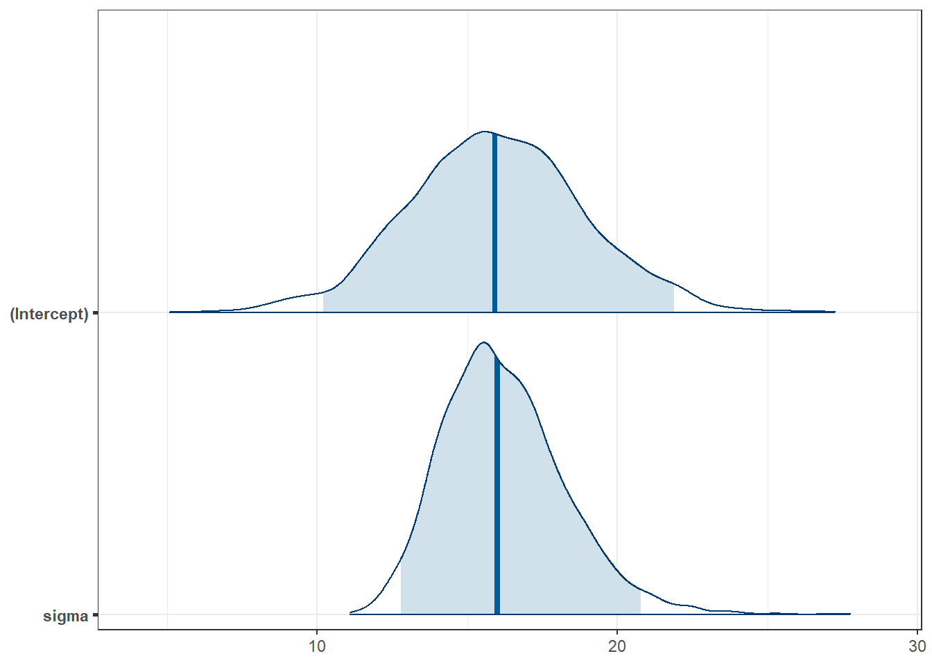

fit6 |>
  model_parameters() |>
  kable(digits = 2)

Parameter	Median	CI	CI_low	CI_high	pd	Rhat	ESS	Prior_Distribution	Prior_Location	Prior_Scale
(Intercept)	15.91	0.95	10.2	21.88	1	1	2481.47	normal	15.97	39.66

5.7 Wilcoxon signed rank test

A rank-based procedure called the Wilcoxon signed rank test can also be used to yield a confidence interval statement about the population pseudo-median, a measure of the population distribution’s center (but not the population’s mean).

Sometimes, a non-parametric alternative is desirable if the data are symmetric (in the sense that the mean and median are close) but show substantial differences in tail behavior from a Normal distribution. In that case, you will often see a report of a Wilcoxon signed rank test, as shown below:

wilcox.test(difference ~ 1, data = bloodlead,
  conf.int = TRUE, conf.level = 0.95, exact = FALSE)

    Wilcoxon signed rank test with continuity correction

data:  difference
V = 499, p-value = 1.155e-05
alternative hypothesis: true location is not equal to 0
95 percent confidence interval:
  9.999943 21.499970
sample estimates:
(pseudo)median 
      15.49996 

As it turns out, if you’re willing to assume the population is symmetric (but not necessarily Normally distributed) then the population pseudo-median is actually equal to the population median.

Note that the pseudo-median here (15.5) is actually slightly closer here to the sample mean (15.97) than it is to the sample median (15).

There are two problems with the Wilcoxon signed-rank approach which make it something I use very rarely in practical work.

1. Converting the data to ranks is a strong transformation that loses a lot of the granular information in the data.
2. The parameter estimated here, called the pseudo-median is not the same as either the sample mean or sample median, and is thus a challenge to interpret.

As a result, bootstrap approaches, though more computationally intricate, are usually better choices for my work.

Note

The pseudo-median of a particular distribution G is the median of the distribution of (u + v)/2, where both u and v have the same distribution (G).

• If the distribution G is symmetric, then the pseudomedian is equal to the median.
• If the distribution is skewed, then the pseudomedian is not the same as the median.
• For any sample, the pseudomedian is defined as the median of all of the midpoints of pairs of observations in the sample.

5.8 Sign test

We can also answer the question: How many of the paired differences (out of the 33 pairs) are positive?

bloodlead |> count(exposed > control)

# A tibble: 2 × 2
  `exposed > control`     n
  <lgl>               <int>
1 FALSE                   5
2 TRUE                   28

and here is a reasonably appropriate 95% confidence interval for this proportion.

binom.test(x = 28, n = 33, conf.level = 0.95)

    Exact binomial test

data:  28 and 33
number of successes = 28, number of trials = 33, p-value = 6.619e-05
alternative hypothesis: true probability of success is not equal to 0.5
95 percent confidence interval:
 0.6810102 0.9489113
sample estimates:
probability of success 
             0.8484848 

The confidence interval provided doesn’t relate back to our original population means. It’s just showing the confidence interval around the probability of the exposed mean being greater than the control mean for a pair of children. We’ll return to studying confidence intervals for proportions in Chapter 13.

5.9 Comparing the Results

Method	Point Estimate	95% Uncertainty Interval
Linear fit (lm)	\(\bar{x} = 15.97\)	(10.34, 21.59)
t test	\(\bar{x} = 15.97\)	(10.34, 21.59)
Bootstrap mean	\(\bar{x} = 15.97\)	(10.79, 21.34)
Bootstrap median	median(x) = 15	(6.98, 23)
Bayesian fit	\(\bar{x} = 15.91\)	(10.20, 21.88)
Signed Rank	pseudo-med(x) = 15.5	(10, 21.5)

Do you see large differences here? Is it surprising that the Bayesian fit’s estimates are closer to 0 than the linear fit?

5.9.1 Assumptions

1. All approaches assume that the data are independent samples from a distribution of paired differences in blood lead levels.
2. All approaches work better with larger samples.
3. All approaches assume that the paired differences are a random sample from a population or process with a fixed distribution of such differences.
4. The linear fit assumes the distribution of differences can be modeled well by a Normal distribution, as does the equivalent t-test.
5. The Wilcoxon signed rank test assumes a symmetric distribution, but not necessarily a Normal one.
6. The bootstrap has even more minor distributional requirements, essentially requiring only that the mean (or median) be an appropriate choice of summary for the center of the distribution.
7. The Bayesian assumptions also include a set of weakly informative prior distributions for the parameters in the model.

None of the methods dominates all of the rest. We will focus most of our effort in this book on least squares linear models fit with lm() and on Bayesian alternatives fit with stan_glm().

5.9.2 General Advice

We have described several approaches to estimating a confidence interval for the center of a distribution of quantitative data.

1. The most commonly used approach uses the t distribution to estimate a confidence interval for a population/process mean. This requires some extra assumptions, most particularly that the underlying distribution of the population values is at least approximately Normally distributed. This is identical to the result we get from an intercept-only linear regression model.

2. A more modern and very general approach uses the idea of the bootstrap to estimate a confidence for a population/process parameter, which could be a mean, median or other summary statistic. The bootstrap, and the underlying notion of resampling is an important idea that lets us avoid some of the assumptions (in particular Normality) that are required by other methods. Bootstrap confidence intervals involve random sampling, so that the actual values obtained will differ a bit across replications.

3. A Bayesian linear model can be used to fit credible intervals, and has some advantages and disadvantages as compared to the intercept-only least squares fit.

4. The Wilcoxon signed-rank method is one of a number of inferential tools which transform the data to their ranks before estimating a confidence interval. This avoids some assumptions, but yields inferences about a less-familiar parameter - the pseudo-median.

Most of the time, the bootstrap provides a reasonably adequate confidence interval estimate of the population value of a parameter (mean or median, most commonly) from a distribution when our data consists of a single sample of quantitative information.

5.10 For More Information

1. The infer package has a nice place to get started at Getting to know infer.

2. Relevant sections of OpenIntro Stats (pdf) include:

• Section 7 - inference for numerical data (except we postpone most of the ideas in section 7.4 until 432.)

Cohen, Jacob. 1988. Statistical Power Analysis for the Behavioral Sciences. 2nd ed. New York: Routledge. https://www.utstat.toronto.edu/~brunner/oldclass/378f16/readings/CohenPower.pdf.

Morton, D., A. Saah, S. Silberg, W. Owens, M. Roberts, and M. Saah. 1982. “Lead Absorption in Children of Employees in a Lead Related Industry.” American Journal of Epidemiology 115: 549–55.

Pruzek, Robert M., and James E. Helmreich. 2009. “Enhancing Dependent Sample Analyses with Graphics.” Journal of Statistics Education 17(1). http://ww2.amstat.org/publications/jse/v17n1/helmreich.html.