4  Data Wrangling

4.1 R setup for this chapter

Note

This section loads all needed R packages for this chapter. Appendix A lists all R packages used in this book, and also provides R session information. Appendix B describes the 431-Love.R script, and demonstrates its use.

library(janitor)
library(knitr)
library(naniar)

library(easystats)
library(tidyverse)

source("data/Love-431.R")

4.2 Data from a .csv file: Cleveland Neighborhoods

Note

Appendix C provides further guidance on pulling data from other systems into R, while Appendix D gives more information (including download links) for all data sets used in this book.

We will demonstrate ideas in this chapter using a tibble containing information on neighborhoods within the city of Cleveland, Ohio. Here, we ingest the data from a .csv (comma-separated version) file called cle_nbd.csv into an R tibble we’ll call cle_neigh, then print the result.

cle_neigh <- read_csv("data/cle_nbd.csv",
  show_col_types = FALSE
)

cle_neigh

# A tibble: 34 × 9
   nbhd_id nbhd_name    pop20 pop10 pop_grow location age65plus income22 unemp22
     <dbl> <chr>        <dbl> <dbl> <chr>    <chr>        <dbl>    <dbl> <chr>  
 1       1 BELLAIRE-PU… 13823 13380 Rise     West         13.8     41324 Middle 
 2       2 BROADWAY-SL… 18854 22331 Fall     Central      11.8     32896 Middle 
 3       3 BROOKLYN CE…  8315  8948 Fall     Central      11.8     32308 Middle 
 4       4 BUCKEYE SHA… 11419 12470 Fall     East         22.5     35402 Middle 
 5       5 CENTRAL      11955 12306 Fall     Central       7.41    16258 High   
 6       6 CLARK FULTON  7625  8509 Fall     Central      10.6     33006 Middle 
 7       7 COLLINWOOD …  9616 11542 Fall     East         13.5     30580 Middle 
 8       8 CUDELL        9125  9287 Fall     West         10.3     29417 High   
 9       9 CUYAHOGA VA…  1404  1371 Rise     Central       1.54    20266 High   
10      10 DETROIT-SHO… 11285 11577 Fall     Central      12.0     45235 Low    
# ℹ 24 more rows

n_miss(cle_neigh)

[1] 0

Key sources for these data were U.S. Census Bureau (2020) and NEOCANDO (2024). The data in the cle_neigh tibble describe each of the 34 neighborhoods (technically statistical planning areas) of the City of Cleveland. For each neighborhood, the cle_neigh tibble contains 9 variables, described in the table below.

Variable	Description
nbhd_id	alphabetical order (1-34) of Cleveland neighborhoods
nbhd_name	name of neighborhood
pop20	Total Population, from Decennial Census 2020
pop10	Total Population, from Decennial Census 2010
pop_grow	Rise if Total population increased from 2010 to 2020, else Fall
location	neighborhood’s geographic location (East, Central or West)
age65plus	% of residents ages 65 and higher, from ACS
income22	Median household income, from ACS
unemp22	Unemployment rate as Low (< 10%), Middle (10-15%), High (above 15%), from ACS

Note

• ACS refers to 5-year estimates from the American Community Survey, covering 2018-2022.

4.3 Key Functions for Managing Data

The dplyr package, part of the tidyverse, provides a set of functions (verbs) which we will use frequently in this course to manage data.

4.3.1 The pipe

There are two main pipes used in R. They are tools for clearer coding that is easier to read, when you are putting multiple steps together into chain.

For example, the code below uses the |> pipe:

cle_neigh |> head()

# A tibble: 6 × 9
  nbhd_id nbhd_name     pop20 pop10 pop_grow location age65plus income22 unemp22
    <dbl> <chr>         <dbl> <dbl> <chr>    <chr>        <dbl>    <dbl> <chr>  
1       1 BELLAIRE-PUR… 13823 13380 Rise     West         13.8     41324 Middle 
2       2 BROADWAY-SLA… 18854 22331 Fall     Central      11.8     32896 Middle 
3       3 BROOKLYN CEN…  8315  8948 Fall     Central      11.8     32308 Middle 
4       4 BUCKEYE SHAK… 11419 12470 Fall     East         22.5     35402 Middle 
5       5 CENTRAL       11955 12306 Fall     Central       7.41    16258 High   
6       6 CLARK FULTON   7625  8509 Fall     Central      10.6     33006 Middle 

applies the head() function to the cle_neigh data. Specifically, the |> pipes the information from the cle_neigh data into the function head(). As we’ll see, we can string a series of pipes together to apply a chain of actions to our data.

The head() function simply shows the first 6 rows of the data, while the tail() function shows the last 6 rows.

Another, similar, pipe is %>%, which does almost the same thing as |> and is read the same way. Here, we pipe the cle_neigh data into the tail() function, and also ask to show the last 8 rows of the data, instead of the default six.

cle_neigh %>% tail(8)

# A tibble: 8 × 9
  nbhd_id nbhd_name     pop20 pop10 pop_grow location age65plus income22 unemp22
    <dbl> <chr>         <dbl> <dbl> <chr>    <chr>        <dbl>    <dbl> <chr>  
1      27 OLD BROOKLYN  32315 32009 Rise     Central      13.3     48061 Middle 
2      28 SAINT CLAIR-…  5139  6876 Fall     East         16.7     29612 Middle 
3      29 STOCKYARDS     9522 10411 Fall     Central      12.3     33553 Middle 
4      30 TREMONT        7699  7975 Fall     Central       9.44    58716 Low    
5      31 UNION-MILES … 15625 19004 Fall     East         20.1     32788 High   
6      32 UNIVERSITY C…  9558  7939 Rise     East         14.9     24780 Low    
7      33 WEST BOULEVA… 18971 18888 Rise     West          9.75    37973 Middle 
8      34 WOODLAND HIL…  5625  6678 Fall     East         19.0     25696 Middle 

Wickham, Çetinkaya-Rundel, and Grolemund (2024) has much more on the pipe in its Pipes section.

4.3.2 select()

We use the select() function to choose specific variables (columns) from our tibble.

cle_neigh |>
  select(nbhd_name, pop_grow)

# A tibble: 34 × 2
   nbhd_name               pop_grow
   <chr>                   <chr>   
 1 BELLAIRE-PURITAS        Rise    
 2 BROADWAY-SLAVIC VILLAGE Fall    
 3 BROOKLYN CENTRE         Fall    
 4 BUCKEYE SHAKER          Fall    
 5 CENTRAL                 Fall    
 6 CLARK FULTON            Fall    
 7 COLLINWOOD NOTTINGHAM   Fall    
 8 CUDELL                  Fall    
 9 CUYAHOGA VALLEY         Rise    
10 DETROIT-SHOREWAY        Fall    
# ℹ 24 more rows

As you can see, this version of the data includes only the two variables we selected.

4.3.3 filter()

In contrast, we use the filter() function to choose specific subjects (rows) from our tibble.

cle_neigh |>
  filter(pop_grow == "Rise" & location == "West")

# A tibble: 5 × 9
  nbhd_id nbhd_name     pop20 pop10 pop_grow location age65plus income22 unemp22
    <dbl> <chr>         <dbl> <dbl> <chr>    <chr>        <dbl>    <dbl> <chr>  
1       1 BELLAIRE-PUR… 13823 13380 Rise     West         13.8     41324 Middle 
2      12 EDGEWATER      6000  5851 Rise     West         13.5     52709 Low    
3      17 HOPKINS         366   215 Rise     West         14.5     29497 Middle 
4      19 JEFFERSON     17351 16548 Rise     West         11.3     49908 Low    
5      33 WEST BOULEVA… 18971 18888 Rise     West          9.75    37973 Middle 

Here, we’ve selected only those rows that have rising population growth and are located in the West.

We can combine filter() and select() to choose both specific rows (here, those with incomes over 50,000) and columns (neighborhood ID code, name, income, unemployment and location.)

cle_neigh |>
  filter(income22 > 50000) |>
  select(nbhd_id, nbhd_name, income22, unemp22, location)

# A tibble: 6 × 5
  nbhd_id nbhd_name     income22 unemp22 location
    <dbl> <chr>            <dbl> <chr>   <chr>   
1      11 DOWNTOWN         61467 Low     Central 
2      12 EDGEWATER        52709 Low     West    
3      20 KAMMS CORNERS    63280 Low     West    
4      22 LEE-HARVARD      53278 Middle  East    
5      26 OHIO CITY        62890 Low     Central 
6      30 TREMONT          58716 Low     Central 

4.3.4 mutate()

We use the mutate() function to create new variables that are combinations of the old ones. For instance, here we create a pop_chg variable which is the percentage change in population from pop10 to pop20.

cle_neigh |>
  mutate(pop_chg = 100 * (pop20 - pop10) / pop20) |>
  select(nbhd_name, pop20, pop10, pop_grow, pop_chg) |>
  tail(4)

# A tibble: 4 × 5
  nbhd_name         pop20 pop10 pop_grow pop_chg
  <chr>             <dbl> <dbl> <chr>      <dbl>
1 UNION-MILES PARK  15625 19004 Fall     -21.6  
2 UNIVERSITY CIRCLE  9558  7939 Rise      16.9  
3 WEST BOULEVARD    18971 18888 Rise       0.438
4 WOODLAND HILLS     5625  6678 Fall     -18.7  

Here, we use the tail(4) function to show the last four rows in this new set of data.

Another common use of mutate() is to create transformations of our data, using functions like the square root, inverse or logarithm.

cle_neigh |>
  mutate(loginc = log(income22)) |>
  ggplot(aes(x = income22, y = loginc, col = location)) +
  geom_point(size = 3) +
  theme_bw()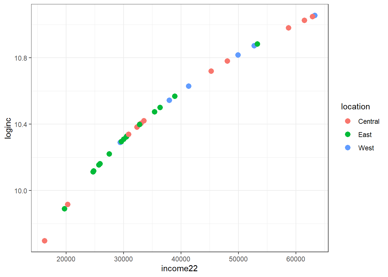

Note that log() is the natural logarithm in R, which we prefer to log10() (the base 10 logarithm) for most of our work because coefficients on the natural log scale will be more easily interpreted, as we’ll see later.

4.3.5 Creating Factors with mutate()

Sometimes we will want to change all of the character variables in a data set into factor variables in R. Factors are used for categorical variables, variables that have a fixed and known set of possible values. They are also useful when you want to display character vectors in a non-alphabetical order. To do so, my favorite approach is:

cle_neigh |>
  mutate(across(where(is.character), as_factor))

# A tibble: 34 × 9
   nbhd_id nbhd_name    pop20 pop10 pop_grow location age65plus income22 unemp22
     <dbl> <fct>        <dbl> <dbl> <fct>    <fct>        <dbl>    <dbl> <fct>  
 1       1 BELLAIRE-PU… 13823 13380 Rise     West         13.8     41324 Middle 
 2       2 BROADWAY-SL… 18854 22331 Fall     Central      11.8     32896 Middle 
 3       3 BROOKLYN CE…  8315  8948 Fall     Central      11.8     32308 Middle 
 4       4 BUCKEYE SHA… 11419 12470 Fall     East         22.5     35402 Middle 
 5       5 CENTRAL      11955 12306 Fall     Central       7.41    16258 High   
 6       6 CLARK FULTON  7625  8509 Fall     Central      10.6     33006 Middle 
 7       7 COLLINWOOD …  9616 11542 Fall     East         13.5     30580 Middle 
 8       8 CUDELL        9125  9287 Fall     West         10.3     29417 High   
 9       9 CUYAHOGA VA…  1404  1371 Rise     Central       1.54    20266 High   
10      10 DETROIT-SHO… 11285 11577 Fall     Central      12.0     45235 Low    
# ℹ 24 more rows

Note that the nbhd_name, pop_grow and unemp22 variables are all now factors in R. We’ll discuss factors in more detail as the semester moves along.

4.3.6 arrange()

cle_neigh |>
  mutate(pop_chg = 100 * (pop20 - pop10) / pop20) |>
  select(nbhd_name, pop20, pop10, pop_grow, pop_chg) |>
  arrange(pop_chg) |>
  head()

# A tibble: 6 × 5
  nbhd_name             pop20 pop10 pop_grow pop_chg
  <chr>                 <dbl> <dbl> <chr>      <dbl>
1 SAINT CLAIR-SUPERIOR   5139  6876 Fall       -33.8
2 GLENVILLE             21137 27394 Fall       -29.6
3 MOUNT PLEASANT        14015 17320 Fall       -23.6
4 UNION-MILES PARK      15625 19004 Fall       -21.6
5 FAIRFAX                5167  6239 Fall       -20.7
6 COLLINWOOD NOTTINGHAM  9616 11542 Fall       -20.0

By default, the arrangement here is sorted from lowest (here, most negative) to highest. To sort from highest to lowest, we could substitute

arrange(desc(pop_chg))

into the code above.

4.3.7 summarise() and group_by()

cle_neigh |>
  group_by(location) |>
  summarise(
    n = n(), mean = mean(income22), sd = sd(income22),
    med = median(income22), mad = mad(income22)
  ) |>
  kable(digits = 2)

location	n	mean	sd	med	mad
Central	12	39628.58	15556.57	33279.5	18509.52
East	15	31038.13	7954.50	30023.0	6415.21
West	7	43444.00	12561.80	41324.0	16879.40

4.4 Describing the Data

Consider the differences between the population in 2020 and the population in 2010 across these neighborhoods.

cle_neigh |>
  reframe(lovedist(pop20 - pop10))

# A tibble: 1 × 10
      n  miss  mean    sd   med   mad   min    q25   q75   max
  <int> <int> <dbl> <dbl> <dbl> <dbl> <dbl>  <dbl> <dbl> <dbl>
1    34     0 -719. 1684.  -519  819. -6257 -1052.  70.5  3838

4.4.1 Are population changes associated with location?

cle_neigh |>
  reframe(lovedist(pop20 - pop10), .by = location)

# A tibble: 3 × 11
  location     n  miss   mean    sd    med   mad   min     q25   q75   max
  <chr>    <int> <int>  <dbl> <dbl>  <dbl> <dbl> <dbl>   <dbl> <dbl> <dbl>
1 West         7     0   101.  487.   149   436.  -758   -39.5  297    803
2 Central     12     0  -171. 1641.  -288.  696. -3477  -696.   101.  3838
3 East        15     0 -1540. 1774. -1053  1014. -6257 -1857   -698   1619

4.4.2 Re-ordering the levels of a factor

cle_neigh |>
  tabyl(unemp22)

 unemp22  n   percent
    High  9 0.2647059
     Low 11 0.3235294
  Middle 14 0.4117647

That’s not so helpful. We really want to show these categories in a natural order (either High then Middle then Low, or the opposite.) We can use the forcats package and the fct_relevel() function to help.

cle_neigh <- cle_neigh |>
  mutate(
    unemp22 =
      fct_relevel(unemp22, "Low", "Middle", "High")
  )

cle_neigh |>
  tabyl(unemp22)

 unemp22  n   percent
     Low 11 0.3235294
  Middle 14 0.4117647
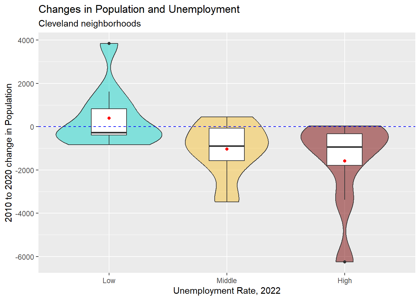
    High  9 0.2647059

4.4.3 Plotting three groups

cle_neigh <- cle_neigh |>
  mutate(pop_diff = pop20 - pop10)

ggplot(data = cle_neigh, aes(
  x = unemp22, y = pop_diff,
  fill = unemp22
)) +
  geom_violin() +
  geom_boxplot(fill = "white", width = 0.3) +
  stat_summary(fun = "mean", geom = "point", col = "red") +
  geom_hline(
    yintercept = 0, col = "blue",
    linetype = "dashed"
  ) +
  scale_fill_viridis_d(
    option = "turbo",
    begin = 0.3, alpha = 0.5
  ) +
  guides(fill = "none") +
  labs(
    title = "Changes in Population and Unemployment",
    y = "2010 to 2020 change in Population",
    x = "Unemployment Rate, 2022",
    subtitle = "Cleveland neighborhoods"
  )

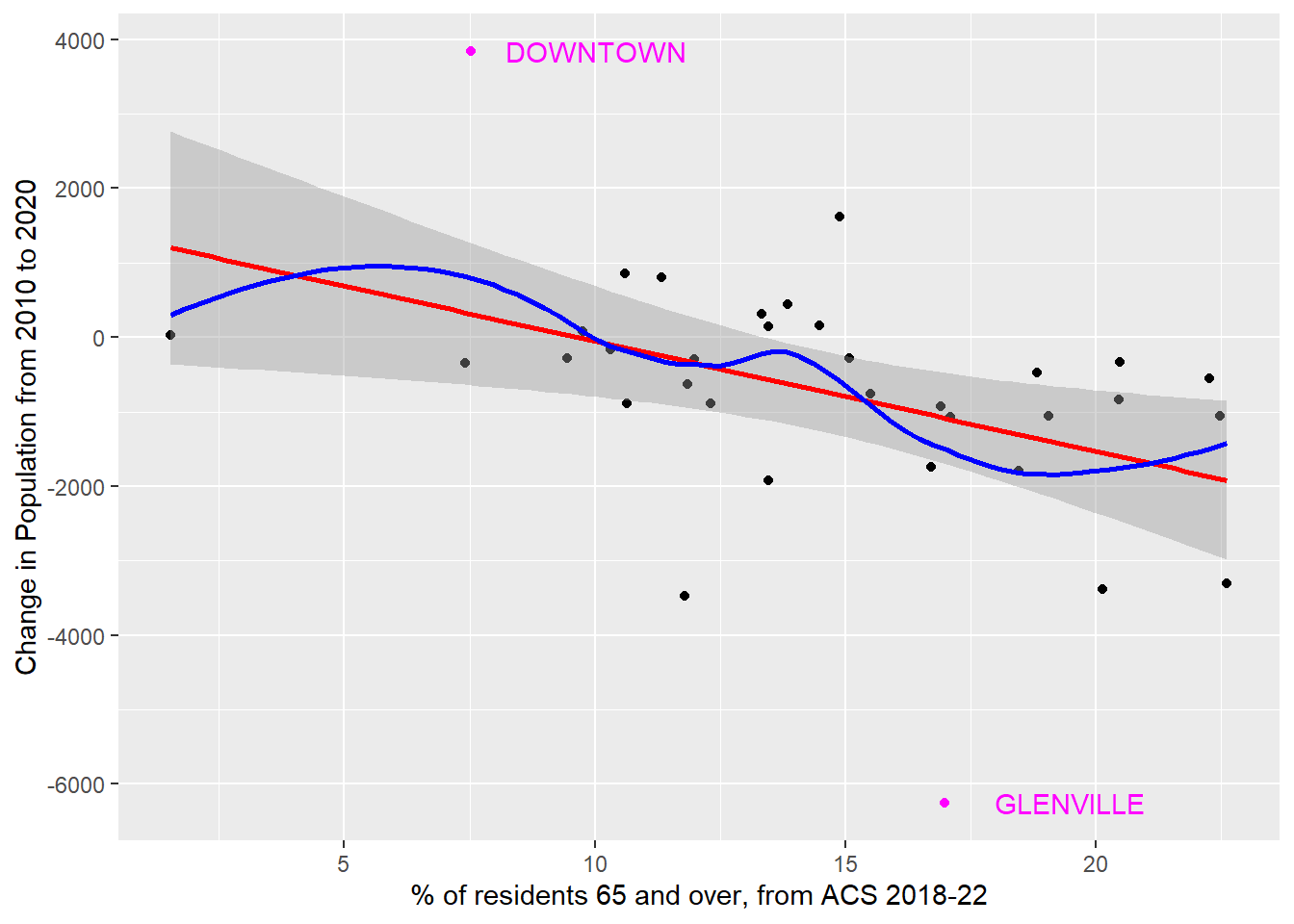
4.4.4 Association of Population Change and % 65+

ggplot(cle_neigh, aes(x = age65plus, y = pop_diff)) +
  geom_point() +
  geom_smooth(
    method = "lm", formula = y ~ x,
    se = TRUE, col = "red"
  ) +
  geom_smooth(
    method = "loess", formula = y ~ x,
    se = FALSE, col = "blue"
  ) +
  geom_text(
    data = cle_neigh |>
      filter(pop_diff > 3000 | pop_diff < -6000),
    aes(label = nbhd_name),
    nudge_x = 2.5, col = "magenta"
  ) +
  geom_point(
    data = cle_neigh |>
      filter(pop_diff > 3000 | pop_diff < -6000),
    col = "magenta"
  ) +
  labs(
    y = "Change in Population from 2010 to 2020",
    x = "% of residents 65 and over, from ACS 2018-22"
  )

4.5 Working with Factors

The forcats package is an important piece of the tidyverse, containing many functions which solve common problems with factors. This PDF cheat sheet is available to help you decide which of the forcats functions might be most useful to help you solve your current problem

Examples of forcats functions that we will use in this course include:

• fct_recode(), which lets us change factor levels by hand
• fct_relevel(), which lets us reorder factor levels by hand
• fct_infreq(), which lets us reorder factor levels by their frequency
• fct_collapse(), which lets us collapse factor levels into manually defined groups
• fct_lump(), which lets us lump uncommon factor levels together into an “other” level

The best place to learn more about factors is the chapter on factors in Wickham, Çetinkaya-Rundel, and Grolemund (2024).

The best place to start learning more about forcats functions is this Introduction to forcats.

4.6 For More Information

1. The dplyr page is a comprehensive source of descriptions for the tools in the dplyr package.

2. The R Graphics Cookbook has an excellent chapter on Getting Your Data into Shape which is well worth your time.

3. R for Data Science (see Wickham, Çetinkaya-Rundel, and Grolemund (2024)) provides an excellent chapter on Data Transformation which goes into further detail on many of the issues discussed here. Other key chapters with something to say about these issues include:

• Workflow: basics
• Code Style and also Data tidying at https://r4ds.hadley.nz/data-tidy
• Factors

4. The datawizard package within the easystats eco-system (see Lüdecke et al. (2022)) has many useful functions.

• In particular, the Coming from Tidyverse page provides a nice vignette describing many of the easystats approaches for wrangling data.

5. The styler package helps to format code according to the tidyverse style guide, which has some appealing features. I try to use this style throughout this book, to improve readability of the work, and I do so by applying a special add-in within R Studio.

Lüdecke, Daniel, Mattan S. Ben-Shachar, Indrajeet Patil, Brenton M. Wiernik, Etienne Bacher, Rémi Thériault, and Dominique Makowski. 2022. “Easystats: Framework for Easy Statistical Modeling, Visualization, and Reporting.” CRAN. https://doi.org/10.32614/CRAN.package.easystats.

NEOCANDO. 2024. “NEOCANDO: Northeast Ohio Community and Neighborhood Data for Organizing.” https://neocando.case.edu/neocando/index.jsp.

U.S. Census Bureau. 2020. “Cleveland, OH City Neighborhoods (Statistical Planning Areas).” https://censusreporter.org/user_geo/70623cc2a11b0ad0e223a2eaa330cf8d/.

Wickham, Hadley, Mine Çetinkaya-Rundel, and Garrett Grolemund. 2024. “R for Data Science, 2e.” https://r4ds.hadley.nz/.