18 Multiple Regression

This is a DRAFT version of this Chapter.

This is a sketchy draft. I’ll remove this notice when I post a version of this Chapter that is essentially finished.

18.1 R setup for this chapter

Note

Appendix A lists all R packages used in this book, and also provides R session information. Appendix B describes the 431-Love.R script, and demonstrates its use.

library(broom)
library(car)
library(GGally)
library(knitr)
library(naniar)
library(rstanarm)
library(tidytuesdayR)

library(easystats)
library(tidyverse)

source("data/Love-431.R")
theme_set(theme_bw())

18.2 Child Care Costs from Tidy Tuesday

Note

Appendix C provides further guidance on pulling data from other systems into R, while Appendix D gives more information (including download links) for all data sets used in this book.

The data for this example is a subset of data described at the Tidy Tuesday repository for 2023-05-09, on Child Care Costs.

The data source is the National Database of Childcare Prices.

The National Database of Childcare Prices (NDCP) is the most comprehensive federal source of childcare prices at the county level. The database offers childcare price data by childcare provider type, age of children, and county characteristics. Data are available from 2008 to 2018.

We will focus on the 2018 data at the county level for the US, and we will read in the data using the tidytuesdayR package.

The data we’re interested in comes in two separate files, one called childcare_costs, and the other called counties.

tuesdata <- tidytuesdayR::tt_load("2023-05-09")

--- Compiling #TidyTuesday Information for 2023-05-09 ----

--- There are 2 files available ---

--- Starting Download ---


    Downloading file 1 of 2: `childcare_costs.csv`
    Downloading file 2 of 2: `counties.csv`

--- Download complete ---

childcare_costs <- tuesdata$childcare_costs
counties <- tuesdata$counties

head(childcare_costs)

# A tibble: 6 × 61
  county_fips_code study_year unr_16 funr_16 munr_16 unr_20to64 funr_20to64
             <dbl>      <dbl>  <dbl>   <dbl>   <dbl>      <dbl>       <dbl>
1             1001       2008   5.42    4.41    6.32        4.6         3.5
2             1001       2009   5.93    5.72    6.11        4.8         4.6
3             1001       2010   6.21    5.57    6.78        5.1         4.6
4             1001       2011   7.55    8.13    7.03        6.2         6.3
5             1001       2012   8.6     8.88    8.29        6.7         6.4
6             1001       2013   9.39   10.3     8.56        7.3         7.6
# ℹ 54 more variables: munr_20to64 <dbl>, flfpr_20to64 <dbl>,
#   flfpr_20to64_under6 <dbl>, flfpr_20to64_6to17 <dbl>,
#   flfpr_20to64_under6_6to17 <dbl>, mlfpr_20to64 <dbl>, pr_f <dbl>,
#   pr_p <dbl>, mhi_2018 <dbl>, me_2018 <dbl>, fme_2018 <dbl>, mme_2018 <dbl>,
#   total_pop <dbl>, one_race <dbl>, one_race_w <dbl>, one_race_b <dbl>,
#   one_race_i <dbl>, one_race_a <dbl>, one_race_h <dbl>, one_race_other <dbl>,
#   two_races <dbl>, hispanic <dbl>, households <dbl>, …

First, we work with the childcare_costs data to select the study_year of 2018, then collect the following variables (besides the county_fips_code we’ll use to link to the counties data and the study_year):

Our outcome will be mfcc_preschool (Aggregated weekly, full-time median price charged for Family Childcare for preschoolers (i.e. aged 36 through 54 months).
Our first predictor is mhi_2018 (Median household income expressed in 2018 dollars.) but recast as mhi_18 (mhi_2018 / 1000) to express income in thousands of 2018 dollars,
Our other predictor is emp_service (Percent of civilians employed in service occupations aged 16 years old and older in the county.)

In terms of dealing with missingness, we will drop all counties with missing values of the outcome, which is the only missing element .

costs <- childcare_costs |>
  filter(study_year == 2018) |>
  mutate(mhi_18 = mhi_2018/1000) |>
  select(county_fips_code, mfcc_preschool, mhi_18, emp_service) |>
  filter(complete.cases(mfcc_preschool))

prop_miss_case(costs)

[1] 0

Next, we use left_join() to merge the childcare costs and the county information by the county_fips_code.

care_costs <- left_join(costs, counties, by = "county_fips_code") |>
  rename(fips = county_fips_code,
         county = county_name,
         state = state_abbreviation) |>
  mutate(fips = as.character(fips))

care_costs

# A tibble: 2,348 × 7
   fips  mfcc_preschool mhi_18 emp_service county          state_name state
   <chr>          <dbl>  <dbl>       <dbl> <chr>           <chr>      <chr>
 1 1001           106.    58.8        15.9 Autauga County  Alabama    AL   
 2 1003           109.    56.0        18.1 Baldwin County  Alabama    AL   
 3 1005            77.1   34.2        14.6 Barbour County  Alabama    AL   
 4 1007            87.1   45.3        18.7 Bibb County     Alabama    AL   
 5 1009           112.    48.7        13   Blount County   Alabama    AL   
 6 1011           106.    32.2        17.1 Bullock County  Alabama    AL   
 7 1013           107.    39.1        16.0 Butler County   Alabama    AL   
 8 1015            85.7   45.2        16.8 Calhoun County  Alabama    AL   
 9 1017           116.    39.9        16.0 Chambers County Alabama    AL   
10 1019            64.6   41.0        12.2 Cherokee County Alabama    AL   
# ℹ 2,338 more rows

If we like, we can then partition the data into separate training and testing samples. Here, we’ll put 70% of the rows (counties) in our training sample, and the remaining 30% into the test sample.

set.seed(431)
ccosts_train <- slice_sample(care_costs, prop = 0.7, replace = FALSE)
ccosts_test <- anti_join(care_costs, ccosts_train, by = "fips")

c(nrow(care_costs), nrow(ccosts_train), nrow(ccosts_test))

[1] 2348 1643  705

18.3 Fit model in training sample with `lm`

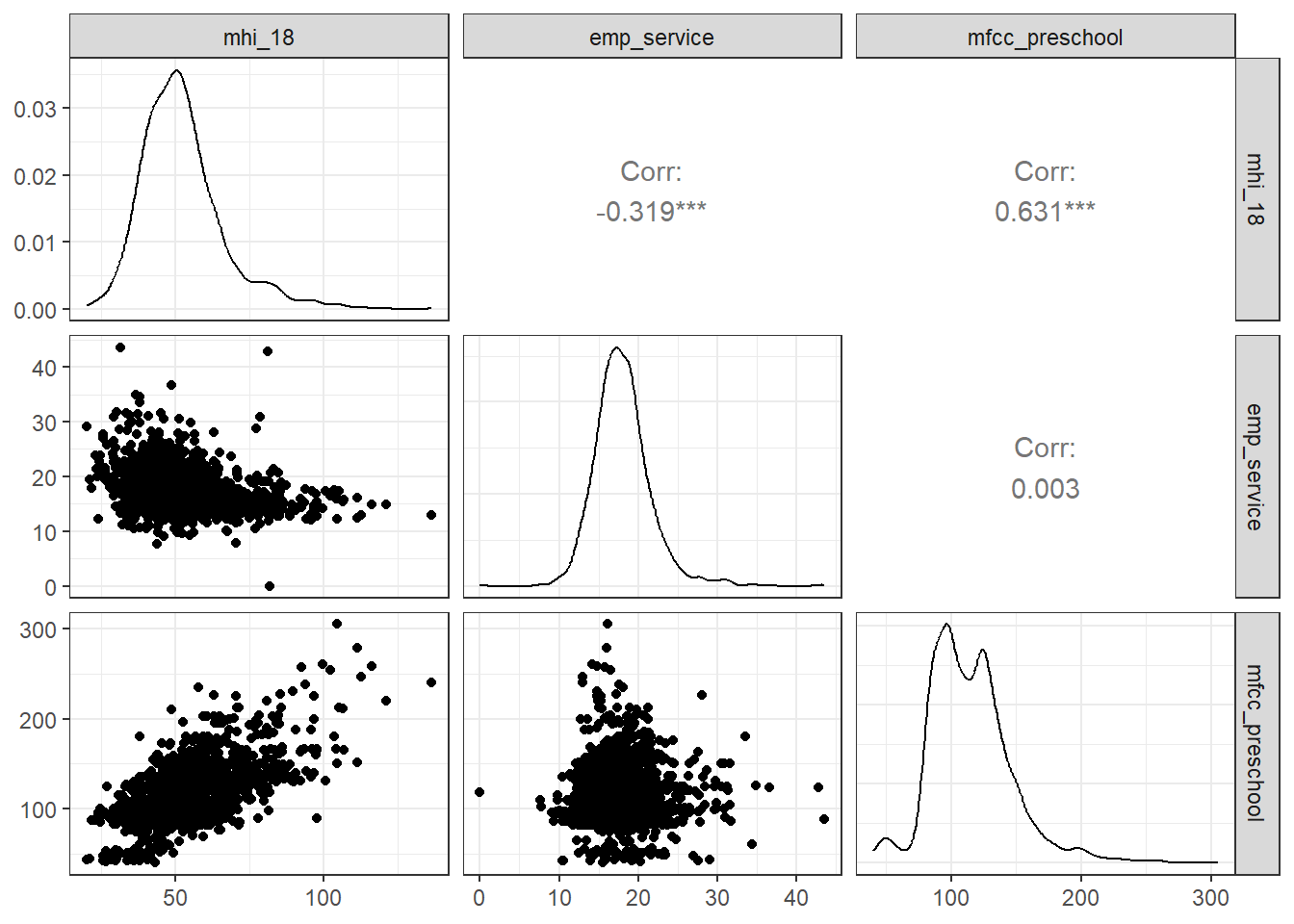
First, draw a picture with ggpairs from GGally of the training sample, so we can see the individual associations.

ggpairs(ccosts_train |> 
          select(mhi_18, emp_service, mfcc_preschool))

Next, we’ll fit the model, and obtain some basic summaries of the model’s parameters and its performance.

fit1 <- lm(mfcc_preschool ~ mhi_18 + emp_service, data = ccosts_train)

model_parameters(fit1, ci = 0.95)

Parameter   | Coefficient |   SE |         95% CI | t(1640) |      p
--------------------------------------------------------------------
(Intercept) |       -3.63 | 4.42 | [-12.30, 5.03] |   -0.82 | 0.411 
mhi 18      |        1.59 | 0.04 | [  1.51, 1.68] |   36.22 | < .001
emp service |        1.99 | 0.17 | [  1.66, 2.33] |   11.69 | < .001


Uncertainty intervals (equal-tailed) and p-values (two-tailed) computed
  using a Wald t-distribution approximation.

model_performance(fit1)

# Indices of model performance

AIC       |      AICc |       BIC |    R2 | R2 (adj.) |   RMSE |  Sigma
-----------------------------------------------------------------------
15063.765 | 15063.789 | 15085.382 | 0.444 |     0.444 | 23.638 | 23.660

Next, we’ll check a set of regression diagnostics to evaluate whether assumptions of linear regression appear to hold sufficiently well.

check_model(fit1)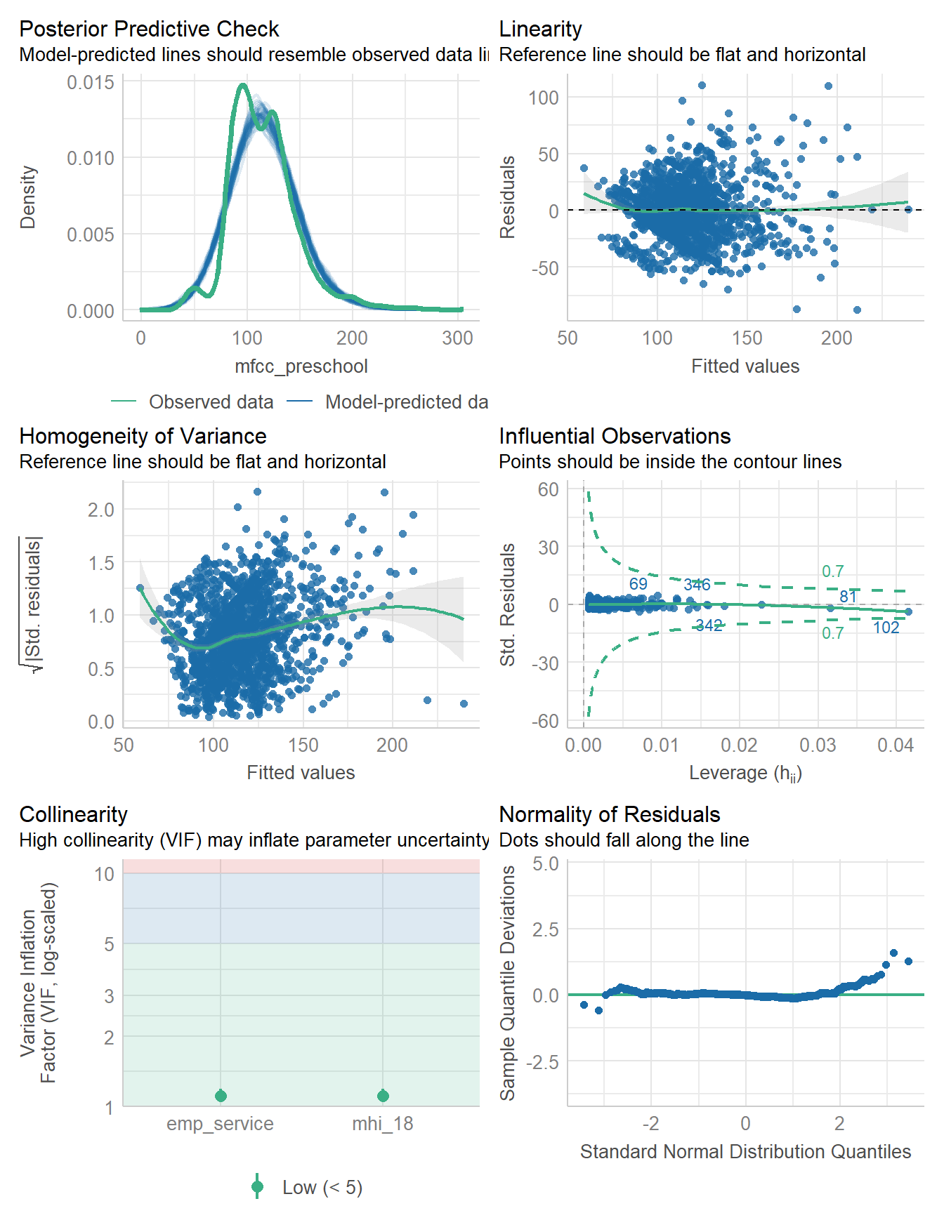

check_heteroscedasticity(fit1)

Warning: Heteroscedasticity (non-constant error variance) detected (p < .001).

check_normality(fit1)

Warning: Non-normality of residuals detected (p < .001).

18.4 Transformation needed?

fit1 <- lm(mfcc_preschool ~ mhi_18 + emp_service, data = ccosts_train)

boxCox(fit1)

18.5 Fitting an alternative model

Here, we’ll also consider fitting a model with only one predictor (the mhi_18) variable, to see whether the addition of emp_service leads to a meaningful improvement. I don’t expect this to be a better model than the model (fit1) that also includes emp_service in this case, but we’ll use this comparison to demonstrate an appealing approach to using training and testing samples.

fit2 <- lm(mfcc_preschool ~ mhi_18, data = ccosts_train)

model_parameters(fit2, ci = 0.95)

Parameter   | Coefficient |   SE |         95% CI | t(1641) |      p
--------------------------------------------------------------------
(Intercept) |       40.81 | 2.35 | [36.21, 45.41] |   17.40 | < .001
mhi 18      |        1.43 | 0.04 | [ 1.34,  1.51] |   32.95 | < .001


Uncertainty intervals (equal-tailed) and p-values (two-tailed) computed
  using a Wald t-distribution approximation.

model_performance(fit2)

# Indices of model performance

AIC       |      AICc |       BIC |    R2 | R2 (adj.) |   RMSE |  Sigma
-----------------------------------------------------------------------
15193.355 | 15193.370 | 15209.568 | 0.398 |     0.398 | 24.604 | 24.619

check_model(fit2)

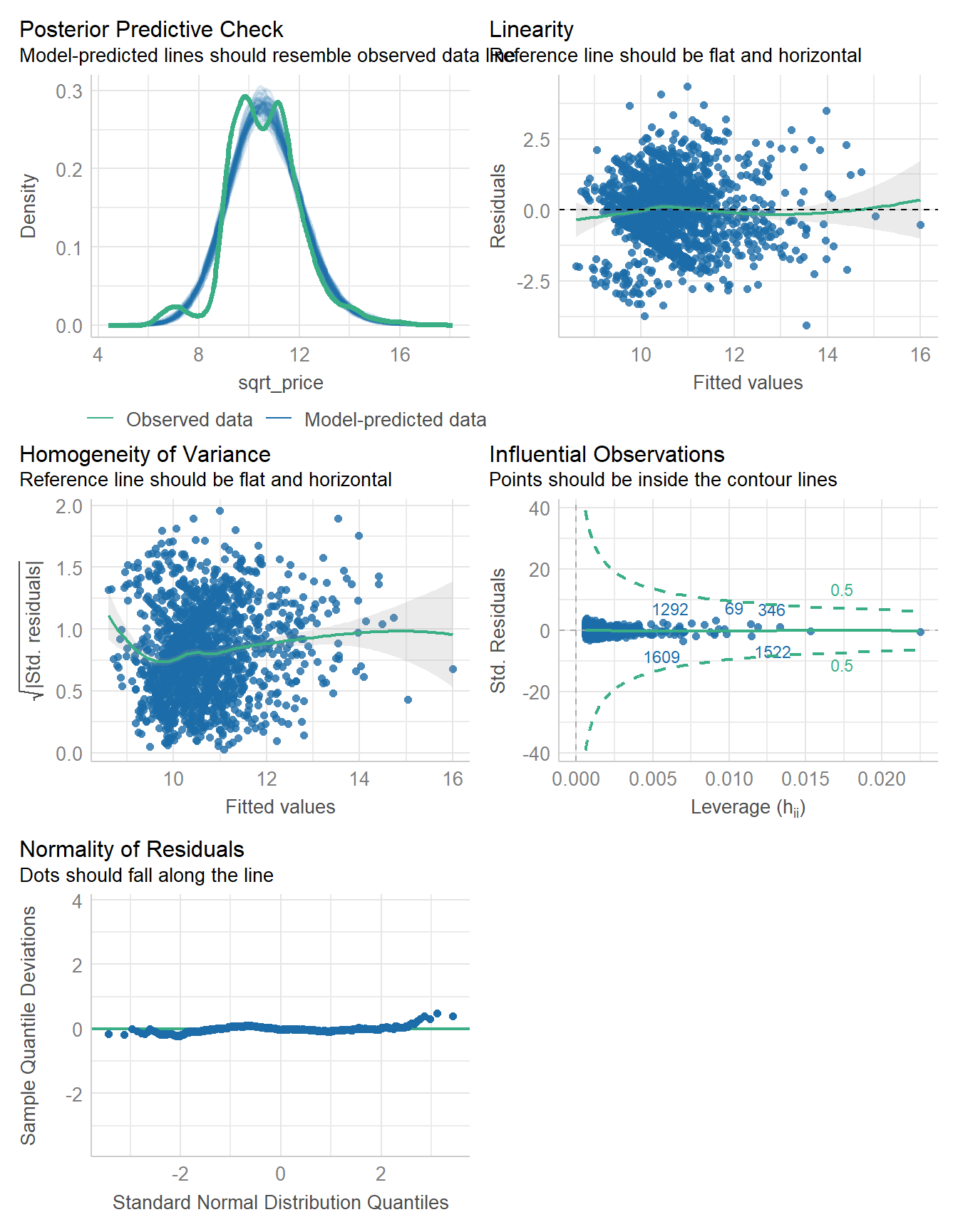
check_heteroscedasticity(fit2)

Warning: Heteroscedasticity (non-constant error variance) detected (p < .001).

check_normality(fit2)

Warning: Non-normality of residuals detected (p < .001).

18.6 Comparing the models (training sample)

We can compare the models within our training sample by comparing the performance statistics, as well as the quality of the diagnostic checks.

compare_performance(fit1, fit2)

# Comparison of Model Performance Indices

Name | Model |   AIC (weights) |  AICc (weights) |   BIC (weights) |    R2 | R2 (adj.) |   RMSE |  Sigma
--------------------------------------------------------------------------------------------------------
fit1 |    lm | 15063.8 (>.999) | 15063.8 (>.999) | 15085.4 (>.999) | 0.444 |     0.444 | 23.638 | 23.660
fit2 |    lm | 15193.4 (<.001) | 15193.4 (<.001) | 15209.6 (<.001) | 0.398 |     0.398 | 24.604 | 24.619

plot(compare_performance(fit1, fit2))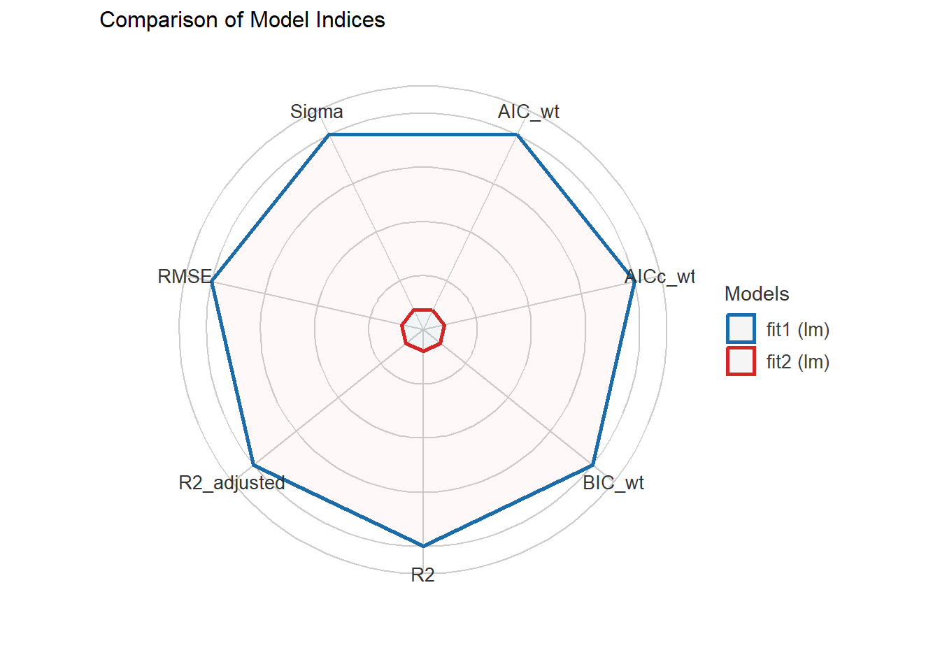

For this “spiderweb” plot, the different indices are normalized and larger values indicate better model performance. So fit2, with points closer to the center displays worse fit indices than fit1 within our training sample. Of course, this isn’t a surprise to us. For more on this, see the documentation online.

18.7 Comparing linear models (test sample)

We’ll use the augment() function from the broom package in this effort.

test1 <- augment(fit1, newdata = ccosts_test) |>
  mutate(mod_n = "Model 1")
test2 <- augment(fit2, newdata = ccosts_test) |>
  mutate(mod_n = "Model 2")

test_res <- bind_rows(test1, test2) |>
  select(mod_n, fips, mfcc_preschool, .fitted, .resid, 
         everything()) |>
  arrange(fips, mod_n)

test_res |> head()

# A tibble: 6 × 10
  mod_n fips  mfcc_preschool .fitted .resid mhi_18 emp_service county state_name
  <chr> <chr>          <dbl>   <dbl>  <dbl>  <dbl>       <dbl> <chr>  <chr>     
1 Mode… 10003           155.    142.  12.7    71.0        16.5 New C… Delaware  
2 Mode… 10003           155.    142.  12.8    71.0        16.5 New C… Delaware  
3 Mode… 10005           122.    130.  -8.38   60.9        18.4 Susse… Delaware  
4 Mode… 10005           122.    128.  -6.11   60.9        18.4 Susse… Delaware  
5 Mode… 1003            109.    122. -13.1    56.0        18.1 Baldw… Alabama   
6 Mode… 1003            109.    121. -12.3    56.0        18.1 Baldw… Alabama   
# ℹ 1 more variable: state <chr>

Now, we can summarize the quality of the predictions across these two models with four summary statistics calculated across the observations in the test sample.

the mean absolute prediction error, or MAPE
the median absolute prediction error, or medAPE
the maximum absolute prediction error, or maxAPE
the square root of the mean squared prediction error, or RMSPE

No one of these dominates the other, but we might be interested in which model gives us the best (smallest) result for each of these summaries. Let’s run them.

test_res |> 
    group_by(mod_n) |>
    summarise(MAPE = mean(abs(.resid)),
              medAPE = median(abs(.resid)),
              maxAPE = max(abs(.resid)),
              RMSPE = sqrt(mean(.resid^2)),
              rsqr = cor(mfcc_preschool, .fitted)^2) |>
  kable()

mod_n	MAPE	medAPE	maxAPE	RMSPE	rsqr
Model 1	17.34671	13.78572	151.2994	23.93467	0.5388358
Model 2	18.16049	13.86123	170.7277	25.37279	0.4738406

Model 1 (including both predictors) performs better within the test sample on each of these four summaries. It has the smaller mean, median and maximum absolute prediction error, and the smaller root mean squared prediction error.

18.8 Bayesian linear model

Here, we’ll demonstrate a Bayesian fit including each of our predictors, with a weakly informative prior, and using the training data.

fit3 <- stan_glm(mfcc_preschool ~ mhi_18 + emp_service, 
                 data = ccosts_train, refresh = 0)

model_parameters(fit3, ci = 0.95)

Parameter   | Median |         95% CI |     pd |  Rhat |     ESS |                    Prior
-------------------------------------------------------------------------------------------
(Intercept) |  -3.55 | [-12.14, 4.66] | 79.15% | 0.999 | 4179.00 | Normal (115.45 +- 79.31)
mhi_18      |   1.59 | [  1.51, 1.68] |   100% | 0.999 | 4659.00 |    Normal (0.00 +- 5.66)
emp_service |   1.99 | [  1.65, 2.32] |   100% | 0.999 | 4568.00 |   Normal (0.00 +- 21.93)


Uncertainty intervals (equal-tailed) and p-values (two-tailed) computed
  using a MCMC distribution approximation.

model_performance(fit3)

# Indices of model performance

ELPD      | ELPD_SE |     LOOIC | LOOIC_SE |      WAIC |    R2 | R2 (adj.) |   RMSE |  Sigma
--------------------------------------------------------------------------------------------
-7532.963 |  35.580 | 15065.927 |   71.160 | 15065.919 | 0.444 |     0.441 | 23.638 | 23.670

check_model(fit3)

18.9 For More Information

431-book Chapter 18 reference OpenStats https://www.openintro.org/book/os/Section 9 - multiple regression (except we don’t do 9.5 in 431)

18.1 R setup for this chapter

18.2 Child Care Costs from Tidy Tuesday

18.3 Fit model in training sample with lm

18.4 Transformation needed?

18.5 Fitting an alternative model

18.6 Comparing the models (training sample)

18.7 Comparing linear models (test sample)

18.8 Bayesian linear model

18.9 For More Information

18.3 Fit model in training sample with `lm`