7 Transformation
7.1 R setup for this chapter
Appendix A lists all R packages used in this book, and also provides R session information. Appendix B describes the 431-Love.R script, and demonstrates its use.
7.2 Data from an .Rds file: DARWIN data
Appendix C provides further guidance on pulling data from other systems into R, while Appendix D gives more information (including download links) for all data sets used in this book.
The DARWIN dataset (Diagnosis AlzheimeR WIth haNdwriting) includes handwriting data specifically designed for the early detection of Alzheimer’s disease (AD). These data are found in the UC Irvine Machine Learning Repository and are derived from Cilia et al. (2022). Gathered into our darwin.Rds file are times to complete three handwriting tasks sampled from the original protocol of 25 such tasks:
- task 1 (a signature),
- task 3 (joining points with a vertical line four times) and
- task 25 (copying a 110-character paragraph)
The .Rds file we have is an R data set, which we can ingest directly with read_rds().
darwin <- read_rds("data/darwin.Rds")

darwin
# A tibble: 174 × 5
subject status time01 time03 time25
<chr> <fct> <dbl> <dbl> <dbl>
1 S_001 HC 5870 10845 61885
2 S_002 AD 7840 12260 41990
3 S_003 AD 156085 20205 159395
4 S_004 AD 4160 3190 77170
5 S_005 HC 6870 10400 124760
6 S_006 AD 5685 5455 252180
7 S_007 HC 5790 2195 36845
8 S_008 AD 8445 10735 106760
9 S_009 AD 9450 24140 72085
10 S_010 AD 17625 8790 122115
# ℹ 164 more rowsn_miss(darwin)[1] 0Our data describe 5 characteristics, including a subject ID (subject) for each of 174 study participants. While the units of time are not clearly specified, they seem to be milliseconds, so, for example, the first subject completed task 1 in 5.87 seconds (5870 ms.) We see also that there are no missing values in the darwin data.
Note that the status variable takes two values:
- HC for Healthy Control
- AD for subject with Alzheimer’s Disease.
darwin |> count(status)# A tibble: 2 × 2
status n
<fct> <int>
1 HC 85
2 AD 89In the rest of this chapter, we will explore the comparison of each of the three task times (gathered in time01, time03 and time 25) between the subjects with Alzheimer’s Disease and the Healthy Controls.
7.3 Visualizing the data for Task 3
In looking at the data for Task 3, we have two independent samples of an outcome (time03) split into two groups by status.
darwin |>
  reframe(lovedist(time03), .by = status)
# A tibble: 2 × 11
status n miss mean sd med mad min q25 q75 max
<fct> <int> <int> <dbl> <dbl> <dbl> <dbl> <dbl> <dbl> <dbl> <dbl>
1 HC 85 0 7477. 4297. 6585 3306. 460 4830 9390 32795
2 AD 89 0 13589. 8183. 12070 7502. 895 7180 17605 39545A plot of the data, like the one below, shows some right skew within each group, specifically a few times that are much longer than the rest. Does a comparison of sample means (shown as gold dots) seem particularly appropriate in this setting?
ggplot(darwin, aes(y = status, x = time03, fill = status)) +
  stat_slab(aes(thickness = after_stat(pdf * n)), scale = 0.7) +
  stat_dotsinterval(side = "bottom", scale = 0.7, slab_linewidth = NA) +
  stat_summary(fun = mean, geom = "point", size = 3, col = "gold") +
  scale_fill_metro_d() +
  guides(fill = "none") +
  labs(x = "Time to complete Task 3 (in ms)")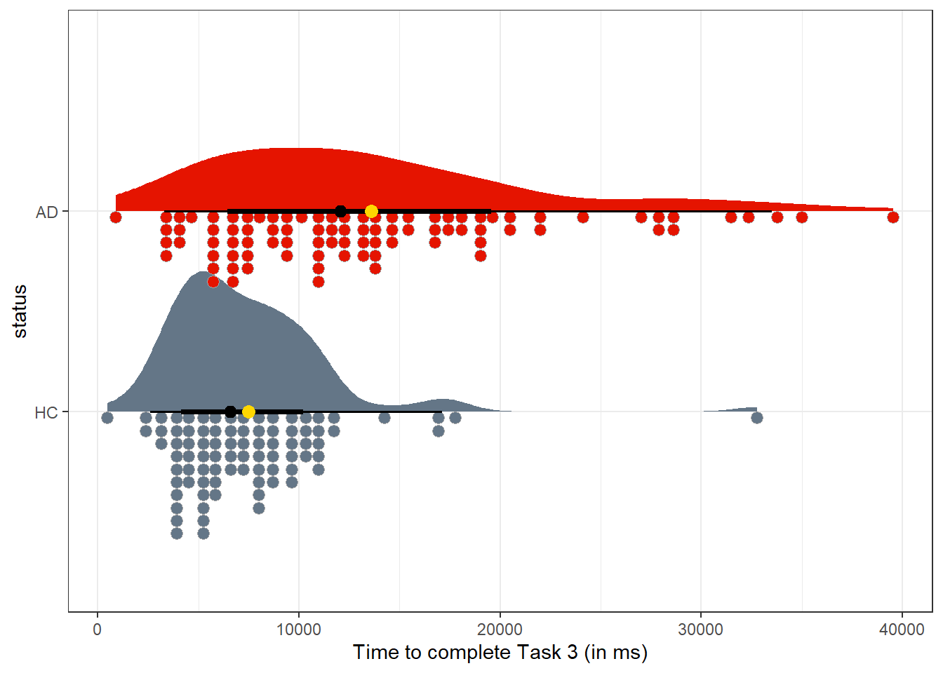
Our approaches for inference about two independent samples mostly anticipate a more symmetric distribution (with less substantial outliers and with the mean closer to the median) in each sample. Could we transform the data on time to complete Task 3 so as to obtain a comparison which might fit those assumptions?
7.4 Some Linear Transformations
Some commonly used transformations in statistics do not change the shape of our distribution in any meaningful way. These are linear transformations, where our transformed data is just a linear function of the original data.
Examples include:
-
centering the data, by subtracting away its mean, so that the mean value of our transformed data becomes zero, which can be accomplished with the
center()function from thedatawizardpackage ineasystats.
dat1 <- darwin |> mutate(ctime03 = center(time03))

dat1 |>
  reframe(lovedist(time03)) |>
kable(digits = 2)| n | miss | mean | sd | med | mad | min | q25 | q75 | max |
|---|---|---|---|---|---|---|---|---|---|
| 174 | 0 | 10603.36 | 7239.98 | 8585 | 4866.63 | 460 | 5568.75 | 13443.75 | 39545 |
| n | miss | mean | sd | med | mad | min | q25 | q75 | max |
|---|---|---|---|---|---|---|---|---|---|
| 174 | 0 | 0 | 7239.98 | -2018.36 | 4866.63 | -10143.36 | -5034.61 | 2840.39 | 28941.64 |
-
rescaling the data to a new range, through division by a constant value, which can be accomplished by setting the desired minimum and maximum values with the
rescale()function from thedatawizardpackage ineasystats.
dat1 <- dat1 |> mutate(rstime03 = rescale(time03, to = c(0, 100)))

dat1 |>
  reframe(lovedist(rstime03)) |>
kable(digits = 2)| n | miss | mean | sd | med | mad | min | q25 | q75 | max |
|---|---|---|---|---|---|---|---|---|---|
| 174 | 0 | 25.95 | 18.52 | 20.79 | 12.45 | 0 | 13.07 | 33.22 | 100 |
-
standardizing the data, which involves both subtracting the mean and dividing by the standard deviation, to produce new data with a mean of 0 and a standard deviation of 1 (this is sometimes referred to as Z-scoring or normalization.) Here, we’ll use the
standardize()function from thedatawizardpackage ineasystats.
dat1 <- dat1 |> mutate(ztime03 = standardize(time03))

dat1 |>
  reframe(lovedist(ztime03)) |>
kable(digits = 2)| n | miss | mean | sd | med | mad | min | q25 | q75 | max |
|---|---|---|---|---|---|---|---|---|---|
| 174 | 0 | 0 | 1 | -0.28 | 0.67 | -1.4 | -0.7 | 0.39 | 4 |
Note, however, that none of these linear transformations fix our problem with the shape of our distribution.
p1 <- ggplot(dat1, aes(x = time03, y = status)) +
  geom_boxplot() +
  labs(title = "Original Time03 data")

p2 <- ggplot(dat1, aes(x = ctime03, y = status)) +
  geom_boxplot() +
  labs(title = "Centered Time03 data")

p3 <- ggplot(dat1, aes(x = rstime03, y = status)) +
  geom_boxplot() +
  labs(title = "Rescaled Time03 data")

p4 <- ggplot(dat1, aes(x = ztime03, y = status)) +
  geom_boxplot() +
  labs(title = "Standardized Time03 data")

(p1 + p2) / (p3 + p4) +
  plot_annotation(title = "Linear Transformations don't change the shape of a distribution.")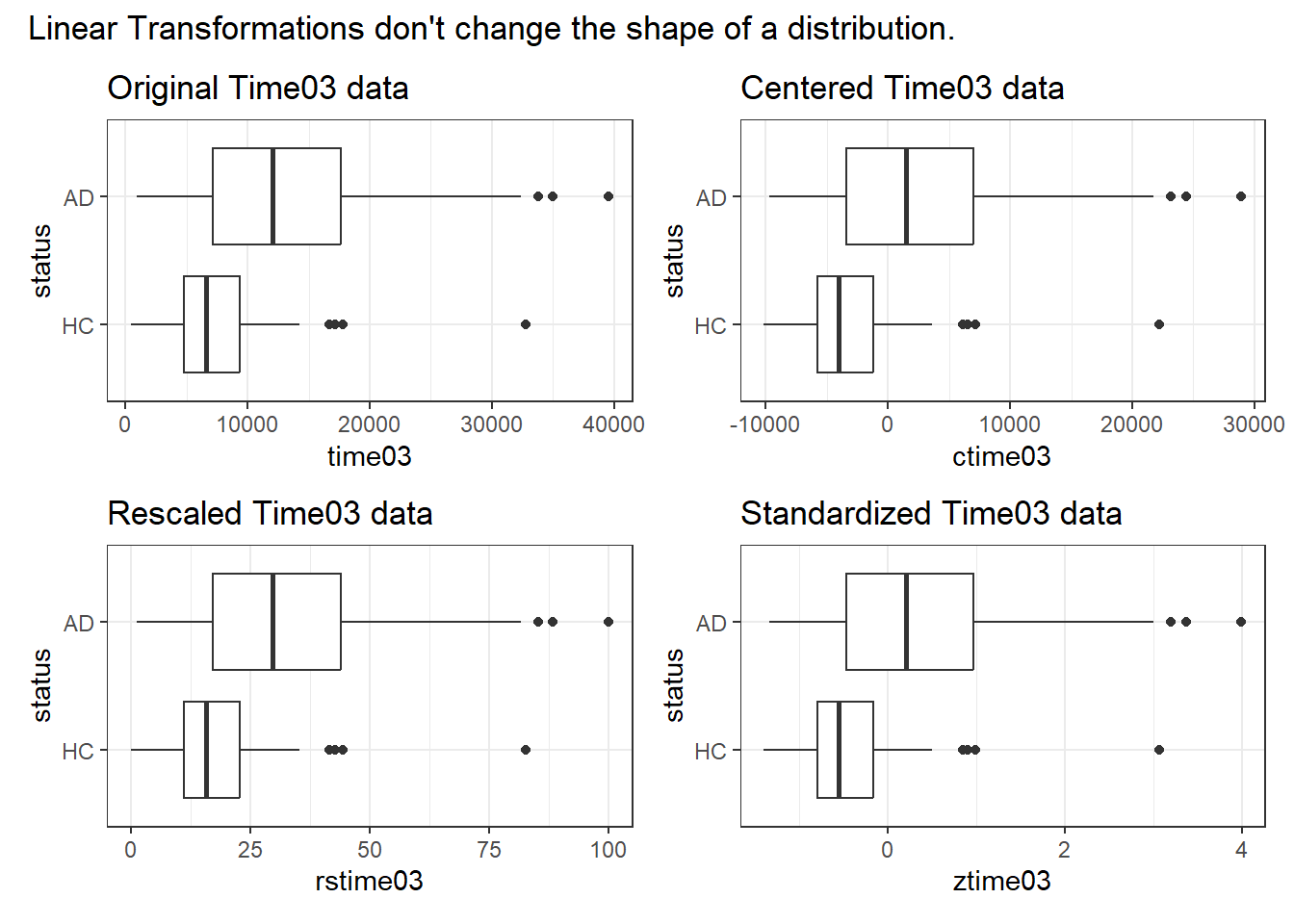
So these linear transformations may slide the distribution back-and-forth along the x axis, and may expand or contract the range of that distribution, but they don’t address the problems we’ve had with the shape of the data.
We need to think about some potential transformations that don’t just add/subtract or multiply/divide by a constant. We need something non-linear.
7.5 The Logarithmic Transformation
The logarithm is one of the more useful non-linear transformations, when our data (as in this case) are entirely positive and show signs of right skew. In R (and in this class), the log() function refers to the natural logarithm, with base \(e\), rather than log10(), which produces the base 10 logarithm. Either can be used to accomplish the same sort of reshaping of our data.
p1 <- ggplot(darwin, aes(x = time03, y = status)) +
  geom_boxplot() +
  stat_summary(geom = "point", fun = "mean", size = 2, col = "red") +
  labs(title = "Original Time03 data")

p2 <- ggplot(darwin, aes(x = log(time03), y = status)) +
  geom_boxplot() +
  stat_summary(geom = "point", fun = "mean", size = 2, col = "red") +
  labs(title = "Natural log of Time03")

p3 <- ggplot(darwin, aes(x = log10(time03), y = status)) +
  geom_boxplot() +
  stat_summary(geom = "point", fun = "mean", size = 2, col = "red") +
  labs(title = "Base 10 log of Time03")

p1 / p2 / p3 +
  plot_annotation(title = "Logarithmic transformations affect the shape of a distribution.")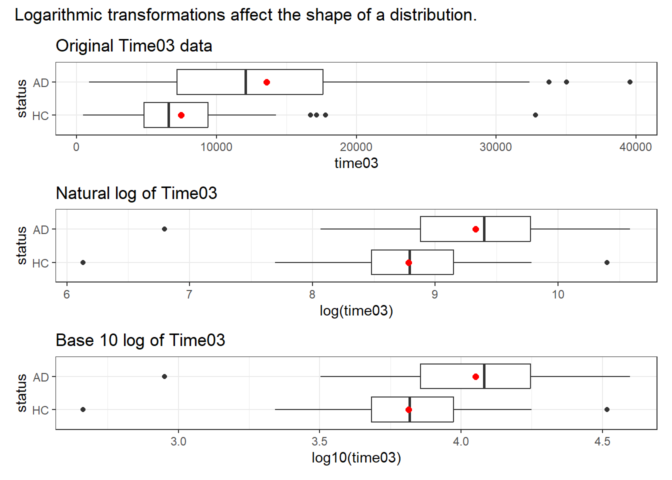
- Each of the logged time distributions are more symmetric (much less right-skewed, with the mean closer to the median) than our original data.
- The two logarithmic bases, though they produce different scales, produce the same distributional shapes as each other.
| status | n | miss | mean | sd | med | mad | min | q25 | q75 | max |
|---|---|---|---|---|---|---|---|---|---|---|
| HC | 85 | 0 | 7476.88 | 4297.36 | 6585 | 3306.20 | 460 | 4830 | 9390 | 32795 |
| AD | 89 | 0 | 13589.33 | 8182.96 | 12070 | 7501.96 | 895 | 7180 | 17605 | 39545 |
| status | n | miss | mean | sd | med | mad | min | q25 | q75 | max |
|---|---|---|---|---|---|---|---|---|---|---|
| HC | 85 | 0 | 8.78 | 0.55 | 8.79 | 0.52 | 6.13 | 8.48 | 9.15 | 10.40 |
| AD | 89 | 0 | 9.33 | 0.66 | 9.40 | 0.66 | 6.80 | 8.88 | 9.78 | 10.59 |
| status | n | miss | mean | sd | med | mad | min | q25 | q75 | max |
|---|---|---|---|---|---|---|---|---|---|---|
| HC | 85 | 0 | 3.81 | 0.24 | 3.82 | 0.22 | 2.66 | 3.68 | 3.97 | 4.52 |
| AD | 89 | 0 | 4.05 | 0.29 | 4.08 | 0.28 | 2.95 | 3.86 | 4.25 | 4.60 |
7.5.1 Importance of the Log Transformation
— from Gelman, Hill, and Vehtari (2021)
The line y = a + bx can be used to express a more general class of relationships by allowing logarithmic transformations. The formula log y = a + bx represents exponential growth (if b > 0) or decline (if b < 0*): y = A exp(bx) where A = exp(a). The parameter A is the value of y when x = 0 and the parameters b determines the rate of growth or decline. A one-unit difference in x corresponds to an additive difference of b in log y and thus a multiplicative factor of exp(b) in y.
It is often helpful to model all-positive random variables on the logarithmic scale because it does not allow for values that are 0 or negative. The logarithmic transformation is non-linear and it pulls in the values at the high end, compressing the scale of the distribution.
7.6 Box-Cox to suggest Power Transformations
There are several other non-linear transformations we might consider in this situation, including an entire family of power distributions. Tukey’s ladder of power transformations can guide our exploration.
| Power (\(\lambda\)) | -2 | -1 | -1/2 | 0 | 1/2 | 1 | 2 |
|---|---|---|---|---|---|---|---|
| Transformation | 1/y2 | 1/y | 1/\(\sqrt{y}\) | log y | \(\sqrt{y}\) | y | y2 |
The Box-Cox plot, sifts through the ladder of options to suggest a transformation (for our outcome) to achieve a more Normal distribution within each group, and linearize the outcome-predictor(s) relationship.
Here’s how we might fit a Box-Cox plot to our data on Task 3.
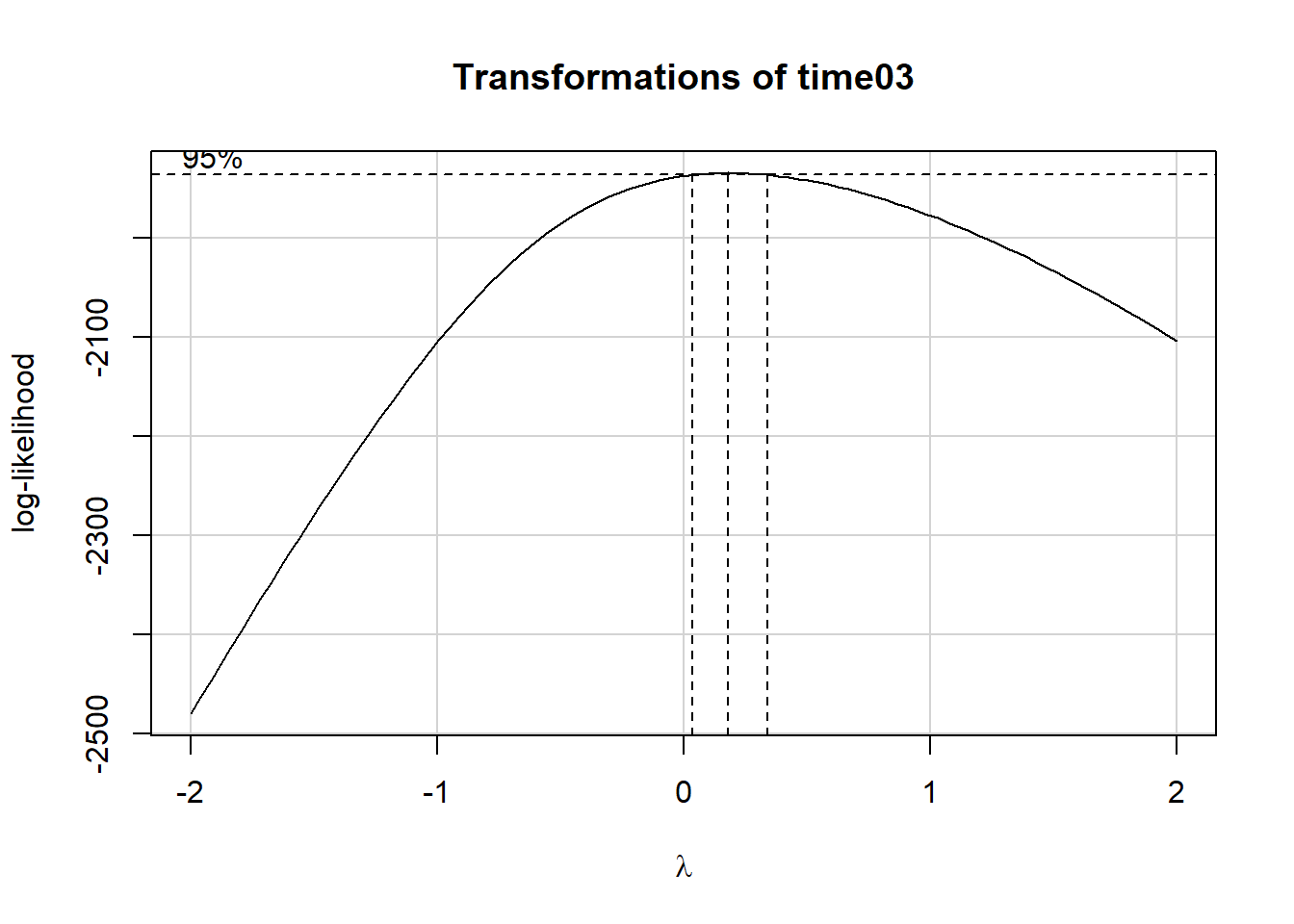
summary(powerTransform(fit3))$result Est Power Rounded Pwr Wald Lwr Bnd Wald Upr Bnd
Y1 0.1836012 0.33 0.03146328 0.3357392The power transformations which the Box-Cox plots suggests here has a power of 0.33, in other words, the cube root of our outcome. But note that the logarithm (power = 0) and square root (power = 0.5) surround this option, and in the interests of simplicity, I’d like to stick to one of those two options. First, I’ll show the log transformation…
p1 <- ggplot(darwin, aes(x = log(time03), y = status)) +
  geom_boxplot() +
  stat_summary(geom = "point", fun = "mean", size = 2, col = "red") +
  labs(title = "Log of Time for Task 3")

p2 <- ggplot(darwin, aes(y = status, x = log(time03), fill = status)) +
  stat_slab(aes(thickness = after_stat(pdf * n)), scale = 0.7) +
  stat_dotsinterval(side = "bottom", scale = 0.7, slab_linewidth = NA) +
  stat_summary(fun = mean, geom = "point", size = 3, col = "gold") +
  scale_fill_metro_d() +
  guides(fill = "none") +
  labs(x = "Log of Time for Task 3")

p1 / p2 +
  plot_annotation(title = "Log of Time for Task 3")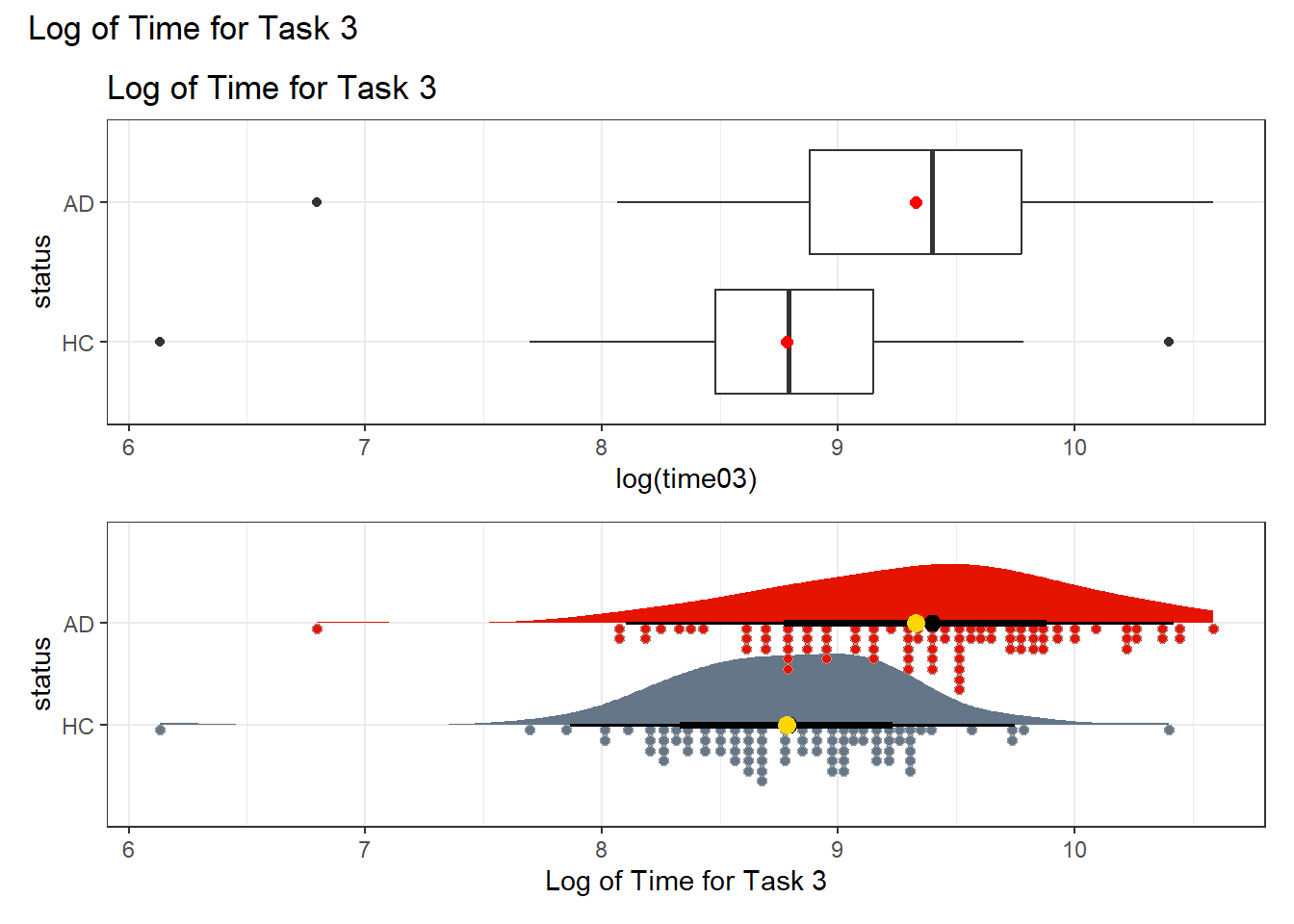
Now, let’s look at the square root transformation instead of the logarithm. Is this a meaningful improvement in terms of adherence to the assumptions required for making a comparison about the means?
p3 <- ggplot(darwin, aes(x = sqrt(time03), y = status)) +
  geom_boxplot() +
  stat_summary(geom = "point", fun = "mean", size = 2, col = "red") +
  labs(title = "Square root of Time for Task 3")

p4 <- ggplot(darwin, aes(y = status, x = sqrt(time03), fill = status)) +
  stat_slab(aes(thickness = after_stat(pdf * n)), scale = 0.7) +
  stat_dotsinterval(side = "bottom", scale = 0.7, slab_linewidth = NA) +
  stat_summary(fun = mean, geom = "point", size = 3, col = "gold") +
  scale_fill_metro_d() +
  guides(fill = "none") +
  labs(x = "Square root of Time for Task 3")

p3 / p4 +
  plot_annotation(title = "Square root of Time for Task 3")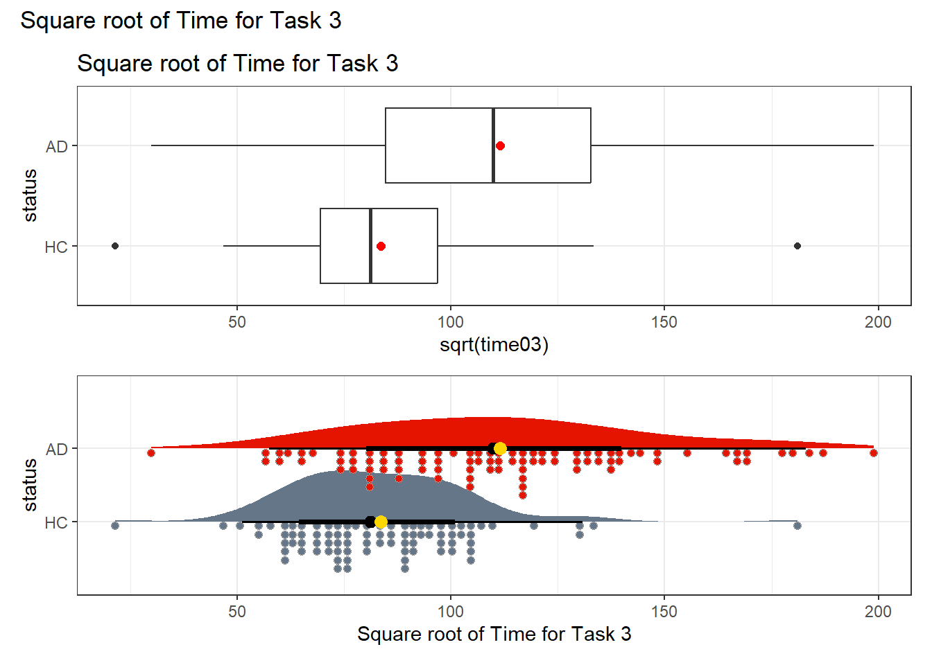
It seems that either transformation (the square root or the logarithm) can do a pretty good job of generating distributions for the two status groups (AD and HC) which are less skewed, and have fewer outliers. I’ll opt to use the logarithm here, because it is such a common choice for transformations in regression, but the square root would also work well in this specific instance.
7.6.1 A Few Caveats
- Some of these transformations (like the logarithm) require the data to be positive. We can rescale the Y data by adding a constant to every observation in a data set without changing shape.
- We can use a natural logarithm (
login R), a base 10 logarithm (log10) or even sometimes a base 2 logarithm (log2) to good effect in Tukey’s ladder. All affect the association’s shape in the same way, so we’ll stick withlog(base e). - Some re-expressions don’t lead to easily interpretable results. Not many things that make sense in their original units also make sense in inverse square roots. There are times when we won’t care, but often, we will.
- If our primary interest is in making predictions, we’ll generally be more interested in getting good predictions back on the original scale, and we can back-transform the point and interval estimates to accomplish this.
7.7 Making Inferences about Task 3
So, we’ll transform our Task 3 times by taking their logarithms.
This produces means in the two exposure groups which are 8.8 and 9.3 for the HC and AD groups, respectively, with standard deviations of 0.55 and 0.66, respectively. It’s appealing to be comparing transformed values which are between 0 and 100 in practice, and so we’ll look to build transformations which accomplish this aim.
7.8 Linear Model and Ordinary Least Squares
To start, we’ll use ordinary least squares and a model fit with lm() to compare the logged times to complete Task 3 across the two status groups.
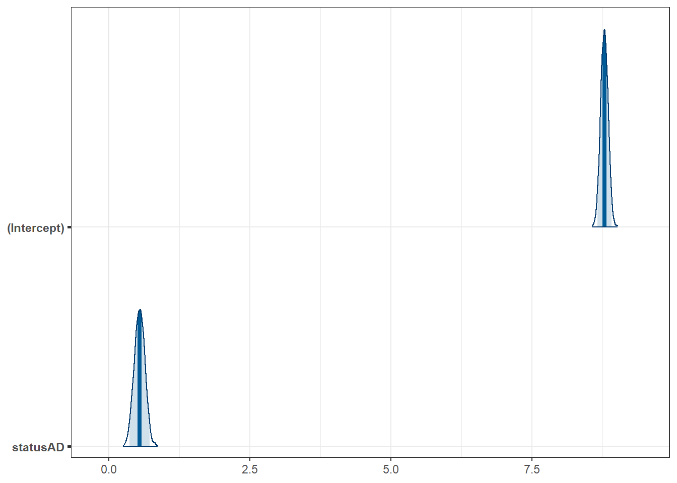
fit3 <- lm(logtime03 ~ status, data = darwin)

fit3 |> model_parameters(ci = 0.95) |>
kable(digits = 2)| Parameter | Coefficient | SE | CI | CI_low | CI_high | t | df_error | p |
|---|---|---|---|---|---|---|---|---|
| (Intercept) | 8.78 | 0.07 | 0.95 | 8.65 | 8.91 | 133.37 | 172 | 0 |
| statusAD | 0.55 | 0.09 | 0.95 | 0.36 | 0.73 | 5.92 | 172 | 0 |
estimate_contrasts(fit3, ci = 0.95, contrast = "status")Marginal Contrasts Analysis
Level1 | Level2 | Difference | SE | 95% CI | t(172) | p
--------------------------------------------------------------------
AD | HC | 0.55 | 0.09 | [0.36, 0.73] | 5.92 | < .001
Variable predicted: logtime03
Predictors contrasted: status
p-values are uncorrected.The AD group has a higher (log time) by about 0.55 with a 95% uncertainty interval of (0.36, 0.73). This transformed time value is no longer expressed in milliseconds, of course, since we’re now talking about a logarithm of time, rather than our original Task 3 time.
7.8.1 Back-transforming the model’s predictions
Your model holds in the “transformed data” world. We cannot back-transform the regression coefficients in a rational way.
After fitting a model, it is useful to generate model-based estimates of the outcomes for different combinations of predictor values, and we can back-transform these predictions to get back to our original scale, as follows.
7.8.1.1 Predictions for The Average Across Many Subjects
If we consider the entire HC group, we would predict that the average log(time03) would be what, exactly?
estimate_expectation(fit3, data = "grid", ci = 0.95) Model-based Predictions
status | Predicted | SE | 95% CI
----------------------------------------
HC | 8.78 | 0.07 | [8.65, 8.91]
AD | 9.33 | 0.06 | [9.20, 9.46]
Variable predicted: logtime03
Predictors modulated: statusThe model fit3 and the estimate_expectation() function can be used to generate expectations for logtime03, which we can then exponentiate to obtain…
- our expectation in terms of the average time to complete Task 3 in milliseconds across all HC subjects, which is 6503 ms (exp(8.78)), with 95% uncertainty interval (5710, 7406) (from exp(8.65), exp(8.91).)
Here, we use R as a calculator…
round_half_up(exp(c(8.78, 8.65, 8.91)),0)[1] 6503 5710 7406Note that the round_half_up() function comes from the janitor package and is an effective way of rounding results for presentation. More on this function is available on the janitor reference page.
- our expectation in terms of the average time to complete Task 3 in milliseconds across all AD subjects turns out to be 11271 ms, with 95% uncertainty interval (9897, 12836).
round_half_up(exp(c(9.33, 9.20, 9.46)),0)[1] 11271 9897 128367.8.1.2 Predictions for Individual Subjects
We can also make predictions for individual subjects with HC or AD, using the estimate_prediction() function applied to our regression model fit3.
estimate_prediction(fit3, data = "grid", ci = 0.95) Model-based Predictions
status | Predicted | SE | 95% CI
-----------------------------------------
HC | 8.78 | 0.61 | [7.58, 9.99]
AD | 9.33 | 0.61 | [8.12, 10.53]
Variable predicted: logtime03
Predictors modulated: status- our prediction of the time an individual HC subject would need to complete Task 3 (in milliseconds) turns out to be 6503 ms, with 95% uncertainty interval (1959, 21807).
round_half_up(exp(c(8.78, 7.58, 9.99)),0)[1] 6503 1959 21807- our prediction of the time an individual AD subject would need to complete Task 3 (in milliseconds) turns out to be 11271 ms, with 95% uncertainty interval (3361, 37421).
round_half_up(exp(c(9.33, 8.12, 10.53)),0)[1] 11271 3361 37421Note how much wider the uncertainty intervals are for individual subjects than for the average across all subjects with a certain status (HC or AD.)
7.8.2 Bootstrap CI for Linear Model Coefficients
Rather than using an OLS fit to obtain the t-distribution based confidence interval for our linear model, we could also bootstrap the confidence intervals in this model with …
model_parameters(fit3, bootstrap = TRUE, iterations = 2000,
  ci = 0.95, centrality = "median", ci_method = "quantile")
Parameter | Coefficient | 95% CI | p
-------------------------------------------------
(Intercept) | 8.78 | [8.66, 8.90] | < .001
status [AD] | 0.55 | [0.36, 0.72] | < .001
Uncertainty intervals (equal-tailed) are naıve bootstrap intervals.7.9 Other approaches
7.9.1 t test (Welch - not pooling SD)
If we run R’s default t test, without assuming equal population variances, on our logged times, we obtain the following, and we’ll also add a calculation of a standardized difference (Cohen’s d) for the effect size (difference in means on the log scale).
fit3a <- t.test(logtime03 ~ status, data = darwin)

fit3a |> model_parameters(ci = 0.95)
Welch Two Sample t-test
Parameter | Group | status = HC | status = AD | Difference | 95% CI
----------------------------------------------------------------------------
logtime03 | status | 8.78 | 9.33 | -0.55 | [-0.73, -0.36]
Parameter | t(169.24) | p
------------------------------
logtime03 | -5.94 | < .001
Alternative hypothesis: true difference in means between group HC and group AD is not equal to 0cohens_d(logtime03 ~ status, data = darwin, pooled_sd = FALSE)Cohen's d | 95% CI
--------------------------
-0.90 | [-1.21, -0.59]
- Estimated using un-pooled SD.7.9.2 t test (with pooled SD)
The t test on our logged times assuming equal variances in the two groups produces the same result as our linear model fit with lm(), of course. Here, though, we can also add a calculation of a standardized difference for the effect size on the log scale.
fit3b <- t.test(logtime03 ~ status, data = darwin, var.equal = TRUE)

fit3b |> model_parameters(ci = 0.95)
Two Sample t-test
Parameter | Group | status = HC | status = AD | Difference | 95% CI
----------------------------------------------------------------------------
logtime03 | status | 8.78 | 9.33 | -0.55 | [-0.73, -0.36]
Parameter | t(172) | p
---------------------------
logtime03 | -5.92 | < .001
Alternative hypothesis: true difference in means between group HC and group AD is not equal to 0cohens_d(logtime03 ~ status, data = darwin, pooled_sd = TRUE)Cohen's d | 95% CI
--------------------------
-0.90 | [-1.21, -0.58]
- Estimated using pooled SD.Because the two groups (HC and AD) have very similar sample sizes and, after transformation, similar standard deviations (and thus similar variances, since the variance is just the square of the standard deviation), it really doesn’t matter whether or not we assume equal variances for these data.
7.9.3 Wilcoxon Signed Rank
We could, instead of transforming the data with the logarithm, use a non-parametric approach to compare the distributions (although this doesn’t compare the means) such as a Wilcoxon signed rank test.
wilcox.test(time03 ~ status, data = darwin,
            conf.int = TRUE, conf.level = 0.95)
    Wilcoxon rank sum test with continuity correction

data:  time03 by status
W = 1829, p-value = 4.105e-09
alternative hypothesis: true location shift is not equal to 0
95 percent confidence interval:
 -6730 -3190
sample estimates:
difference in location
                 -4950
7.9.4 Bayesian linear model
We could also fit a Bayesian linear model to our logged times for Task 3, as follows:
set.seed(431)
fit3c <- stan_glm(logtime03 ~ status, data = darwin, refresh = 0)

post3c <- describe_posterior(fit3c, ci = 0.95)

print_md(post3c, digits = 2)| Parameter | Median | 95% CI | pd | ROPE | % in ROPE | Rhat | ESS |
|---|---|---|---|---|---|---|---|
| (Intercept) | 8.78 | [8.66, 8.91] | 100% | [-0.07, 0.07] | 0% | 1.000 | 3621 |
| statusAD | 0.55 | [0.36, 0.72] | 100% | [-0.07, 0.07] | 0% | 0.999 | 3435 |
fit3c |> model_parameters() |> kable(digits = 2)| Parameter | Median | CI | CI_low | CI_high | pd | Rhat | ESS | Prior_Distribution | Prior_Location | Prior_Scale |
|---|---|---|---|---|---|---|---|---|---|---|
| (Intercept) | 8.78 | 0.95 | 8.66 | 8.91 | 1 | 1 | 3620.57 | normal | 9.06 | 1.66 |
| statusAD | 0.55 | 0.95 | 0.36 | 0.72 | 1 | 1 | 3435.02 | normal | 0.00 | 3.31 |
As with an OLS model fit with lm(), we can back-transform expectations or predictions from this model, but not the coefficients themselves.
estimate_expectation(fit3c, data = "grid", ci = 0.95)Model-based Predictions
status | Predicted | SE | 95% CI
----------------------------------------
HC | 8.78 | 0.07 | [8.66, 8.91]
AD | 9.33 | 0.07 | [9.20, 9.46]
Variable predicted: logtime03
Predictors modulated: statusround_half_up(exp(c(8.78, 8.66, 8.91)),0) # for the mean across HC subjects[1] 6503 5768 7406round_half_up(exp(c(9.33, 9.20, 9.46)),0) # for the mean across AD subjects[1] 11271 9897 12836estimate_prediction(fit3c, data = "grid", ci = 0.95)Model-based Predictions
status | Predicted | SE | 95% CI
-----------------------------------------
HC | 8.79 | 0.60 | [7.58, 9.97]
AD | 9.33 | 0.61 | [8.13, 10.52]
Variable predicted: logtime03
Predictors modulated: statusround_half_up(exp(c(8.79, 7.58, 10.03)),0) # for an individual HC subject[1] 6568 1959 22697round_half_up(exp(c(9.32, 8.12, 10.56)),0) # for an individual AD subject[1] 11159 3361 385617.9.5 Bootstrap CI for mean (time03) without transformation
Finally, we could use the bootstrap directly to build a confidence interval around the difference in means, without using a transformation. The first way I’ll do this uses the tools from the infer package.
set.seed(431)
darwin |>
  specify(time03 ~ status) |>
  generate(reps = 1000, type = "bootstrap") |>
  calculate( stat = "diff in means", order = c("AD", "HC") ) |>
  get_confidence_interval( level = 0.95, type = "percentile" )
# A tibble: 1 × 2
lower_ci upper_ci
<dbl> <dbl>
1 4270. 8048.Or we could use the boot.t.test() approach from the MKinfer package.
set.seed(431)
boot.t.test(time03 ~ status, var.equal = TRUE, R = 2000,
  data = darwin, conf.level = 0.95)
    Bootstrap Two Sample t-test

data:  time03 by status
number of bootstrap samples:  2000
bootstrap p-value < 5e-04
bootstrap difference of means (SE) = -6115.905 (1087.369)
95 percent bootstrap percentile confidence interval:
 -8236.120 -3963.146

Results without bootstrap:
t = -6.1265, df = 172, p-value = 5.94e-09
alternative hypothesis: true difference in means is not equal to 0
95 percent confidence interval:
 -8081.771 -4143.116
sample estimates:
mean in group HC mean in group AD
        7476.882        13589.326
Note the difference between the raw t test result (results without bootstrap) and the bootstrap in this setting.
We can run this without assuming equal population variances, as well.
set.seed(431)
boot.t.test(time03 ~ status, var.equal = FALSE, R = 2000,
  data = darwin, conf.level = 0.95 )
    Bootstrap Welch Two Sample t-test

data:  time03 by status
number of bootstrap samples:  2000
bootstrap p-value < 5e-04
bootstrap difference of means (SE) = -6130.079 (977.7301)
95 percent bootstrap percentile confidence interval:
 -8147.991 -4226.181

Results without bootstrap:
t = -6.2074, df = 134.42, p-value = 6.245e-09
alternative hypothesis: true difference in means is not equal to 0
95 percent confidence interval:
 -8059.950 -4164.937
sample estimates:
mean in group HC mean in group AD
        7476.882        13589.326
7.9.6 Bootstrap CI for Medians
Instead of comparing mean times to complete Task 3, we could use the bootstrap to compare the medians directly.
7.10 What about Task 1?
ggplot(darwin, aes(x = status, y = time01)) +
  geom_boxplot()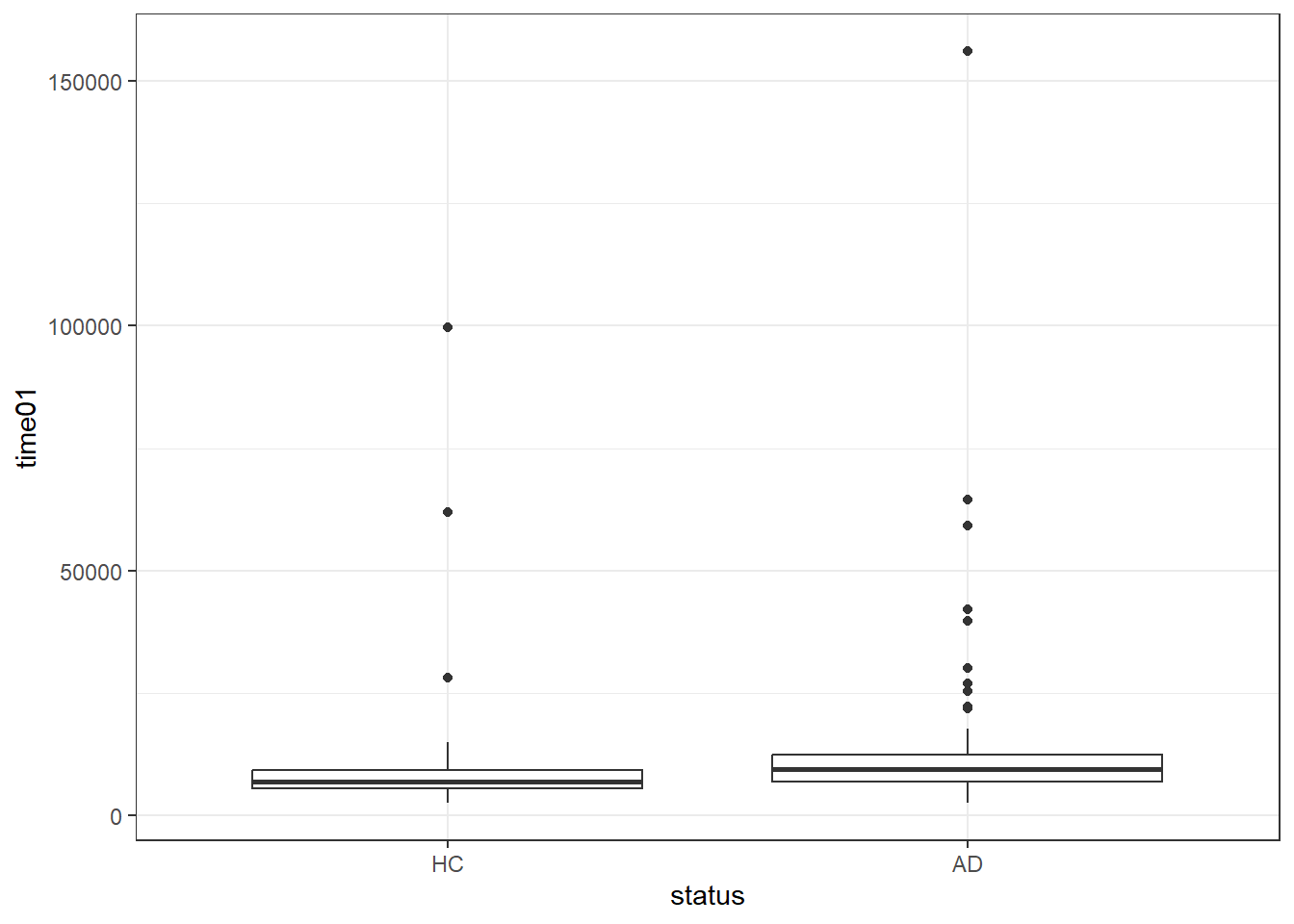
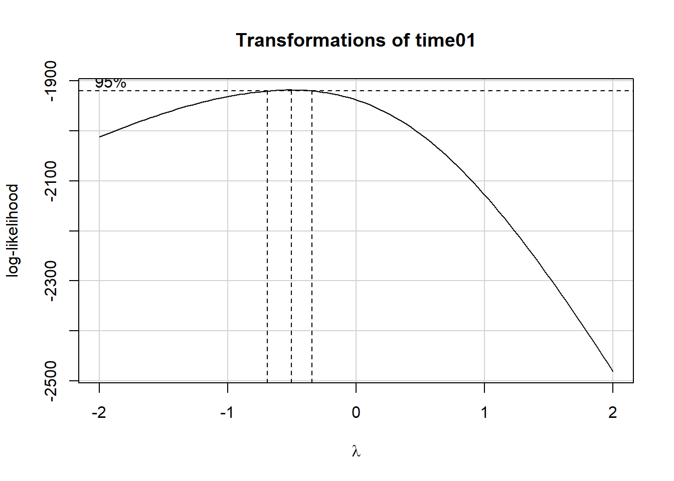
summary(powerTransform(fit1))$result Est Power Rounded Pwr Wald Lwr Bnd Wald Upr Bnd
Y1 -0.5110717 -0.5 -0.6849666 -0.3371769ggplot(darwin, aes(x = status, y = (time01^-0.5))) +
geom_boxplot()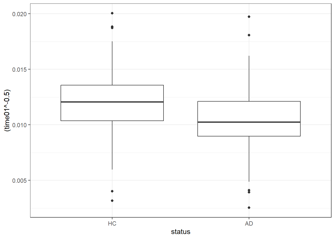
darwin <- darwin |>
  mutate(trans_t01 = 1000 * time01^(-0.5))

darwin |>
  reframe(lovedist(trans_t01), .by = status)
# A tibble: 2 × 11
status n miss mean sd med mad min q25 q75 max
<fct> <int> <int> <dbl> <dbl> <dbl> <dbl> <dbl> <dbl> <dbl> <dbl>
1 HC 85 0 12.0 2.81 12.1 2.37 3.17 10.4 13.6 20.0
2 AD 89 0 10.5 3.05 10.2 2.02 2.53 8.97 12.1 19.77.10.1 Linear Model
fit1 <- lm(trans_t01 ~ status, data = darwin)

fit1 |>
  model_parameters(ci = 0.95) |>
kable(digits = 2)| Parameter | Coefficient | SE | CI | CI_low | CI_high | t | df_error | p |
|---|---|---|---|---|---|---|---|---|
| (Intercept) | 11.98 | 0.32 | 0.95 | 11.36 | 12.61 | 37.64 | 172 | 0 |
| statusAD | -1.45 | 0.45 | 0.95 | -2.33 | -0.57 | -3.25 | 172 | 0 |
estimate_contrasts(fit1, ci = 0.95, contrast = "status")Marginal Contrasts Analysis
Level1 | Level2 | Difference | SE | 95% CI | t(172) | p
---------------------------------------------------------------------
AD | HC | -1.45 | 0.45 | [-2.33, -0.57] | -3.25 | 0.001
Variable predicted: trans_t01
Predictors contrasted: status
p-values are uncorrected.7.10.2 Back-transformation of predictions and expectations…
Here our transformation is trans_t01 = 1000 * time01^(-0.5). To back out of this transformation, we need to do a little algebra…
\[ trans_{t01} = 1000 * time01^{-0.5} \]
\[ trans_{t01} = 1000 * \left(\frac{1}{\sqrt{time01}}\right) \]
\[ \frac{trans_{t01}}{1000} = \left(\frac{1}{\sqrt{time01}}\right) \]
\[ \frac{1000}{trans_{t01}} = \sqrt{time01} \]
\[ \left(\frac{1000}{trans_{t01}}\right)^2 = time01 \]
We can obtain an expectation for trans_t01 from estimate_expectation() and then apply this transformation in order to describe the result in terms of the time to complete Task 1 in milliseconds, as follows…
estimate_expectation(fit1, data = "grid", ci = 0.95)Model-based Predictions
status | Predicted | SE | 95% CI
------------------------------------------
HC | 11.98 | 0.32 | [11.36, 12.61]
AD | 10.54 | 0.31 | [ 9.92, 11.15]
Variable predicted: trans_t01
Predictors modulated: statusSo, for example, our expectation for the average across all HC subjects is 11.98 after our transformation. Backing out of this transformation, we have an estimate of 6968 milliseconds.
round_half_up((1000 / 11.98)^2, 0)[1] 6968To obtain the uncertainty interval for the expectation across all HC subjects, we apply the back-transformation to the endpoints of the interval, and then round the results to no decimal places as follows:
round_half_up(c((1000 / 10.54)^2, (1000 / 9.92)^2, (1000 / 11.15)^2), 0)[1] 9002 10162 8044and so our model’s estimate for the time spent on Task 1 for HC subjects on average is 6968 milliseconds, with a 95% uncertainty interval of (6289, 7749) milliseconds.
For the average across AD subjects, we have a point estimate for the time spent on Task 1 of 9002 ms, and a 95% uncertainty interval of (8044, 10162) ms.
round_half_up(c((1000 / 11.36)^2, (1000 / 12.61)^2), 0)[1] 7749 6289We can obtain analogous results for individual predictions for HC and AD subjects, respectively, according to this model for transformed Task 1 times, with the following code:
estimate_prediction(fit1, data = "grid", ci = 0.95)Model-based Predictions
status | Predicted | SE | 95% CI
-----------------------------------------
HC | 11.98 | 2.95 | [6.16, 17.81]
AD | 10.54 | 2.95 | [4.71, 16.36]
Variable predicted: trans_t01
Predictors modulated: statusround_half_up(c((1000 / 11.98)^2, (1000 / 6.16)^2, (1000 / 17.81)^2), 0) ## HC subjects[1] 6968 26354 3153round_half_up(c((1000 / 10.54)^2, (1000 / 4.71)^2, (1000 / 16.36)^2), 0) ## AD subjects[1] 9002 45077 3736All of our other approaches used for Task 3 would also work for Task 1, certainly.
7.11 What about Task 25?
Finally, let’s consider Task 25.
ggplot(darwin, aes(x = status, y = time25)) +
  geom_boxplot()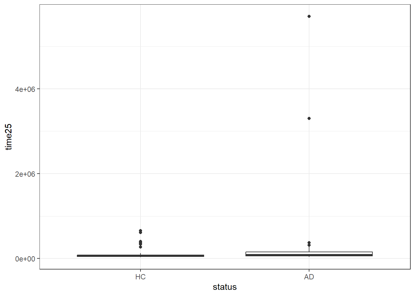
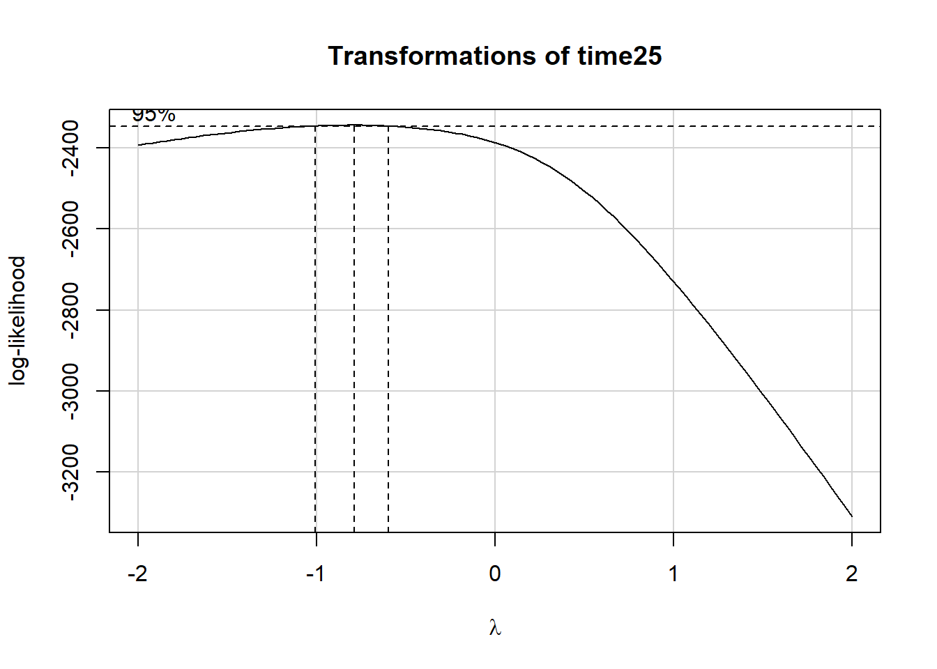
summary(powerTransform(fit25))$result Est Power Rounded Pwr Wald Lwr Bnd Wald Upr Bnd
Y1 -0.7965846 -1 -1.002999 -0.5901699Now, we’ll use an inverse transformation and also multiply the values by 1,000,000 in order to get coefficients which fall between 1 and 100.
ggplot(darwin, aes(x = status, y = (1000000 / time25))) +
  geom_boxplot()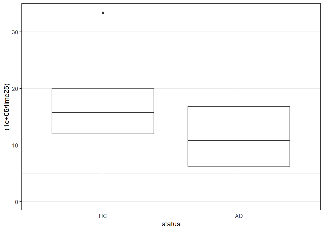
darwin <- darwin |>
  mutate(trans_t25 = 1000000 / time25)

darwin |>
  reframe(lovedist(trans_t25), .by = status)
# A tibble: 2 × 11
status n miss mean sd med mad min q25 q75 max
<fct> <int> <int> <dbl> <dbl> <dbl> <dbl> <dbl> <dbl> <dbl> <dbl>
1 HC 85 0 15.3 6.84 15.8 5.74 1.52 12.0 20.0 33.4
2 AD 89 0 11.0 5.68 10.9 7.19 0.175 6.27 16.8 24.87.11.1 Linear Model
fit25 <- lm(trans_t25 ~ status, data = darwin)

fit25 |> model_parameters(ci = 0.95) |> kable(digits = 2)| Parameter | Coefficient | SE | CI | CI_low | CI_high | t | df_error | p |
|---|---|---|---|---|---|---|---|---|
| (Intercept) | 15.25 | 0.68 | 0.95 | 13.91 | 16.59 | 22.41 | 172 | 0 |
| statusAD | -4.27 | 0.95 | 0.95 | -6.15 | -2.40 | -4.49 | 172 | 0 |
estimate_contrasts(fit25, ci = 0.95, contrast = "status")Marginal Contrasts Analysis
Level1 | Level2 | Difference | SE | 95% CI | t(172) | p
----------------------------------------------------------------------
AD | HC | -4.27 | 0.95 | [-6.15, -2.40] | -4.49 | < .001
Variable predicted: trans_t25
Predictors contrasted: status
p-values are uncorrected.We could also bootstrap the confidence intervals in this model with …
model_parameters(fit25, bootstrap = TRUE, iterations = 2000,
  ci = 0.95, centrality = "median", ci_method = "quantile")
Parameter | Coefficient | 95% CI | p
---------------------------------------------------
(Intercept) | 15.26 | [13.79, 16.68] | < .001
status [AD] | -4.28 | [-6.16, -2.31] | < .001
Uncertainty intervals (equal-tailed) are naıve bootstrap intervals.Working with the original lm() fit, we can obtain predictions or expectations and back-transform them as before. I’ll show the average expectations here…
estimate_expectation(fit25, data = "grid", ci = 0.95)Model-based Predictions
status | Predicted | SE | 95% CI
------------------------------------------
HC | 15.25 | 0.68 | [13.91, 16.59]
AD | 10.98 | 0.67 | [ 9.67, 12.29]
Variable predicted: trans_t25
Predictors modulated: statusHere are the back-transformed point estimate and 95% uncertainty interval for an individual prediction for a subject with status AD to complete Task 25, in milliseconds…
round_half_up(c((1000000 / 10.98), (1000000 / 9.67), (1000000 / 12.29)),0)[1] 91075 103413 81367so the point estimate is 91075 ms, with 95% uncertainty interval (81367, 103413).
However, we run into a challenge when we look at transforming out of the uncertainty interval for individual predictions.
estimate_prediction(fit25, data = "grid", ci = 0.95)Model-based Predictions
status | Predicted | SE | 95% CI
------------------------------------------
HC | 15.25 | 6.31 | [ 2.80, 27.71]
AD | 10.98 | 6.31 | [-1.48, 23.43]
Variable predicted: trans_t25
Predictors modulated: statusFor an individual AD subject, we have:
round_half_up(c((1000000 / 10.98), (1000000 / -1.48), (1000000 / 23.43)),0)[1] 91075 -675676 42680Our 95% uncertainty interval now includes negative times, and the uncertainty interval no longer includes the point estimate, and this causes multiple problems. This suggests that transforming our way out of a problem when making a comparison of this sort is not always going to produce useful results.
7.12 For More Information
Transformation is discussed in some detail as part of this vignette for the
modelbasedpackage vignette from the easystats meta-package.You can learn more about model-based response estimates and uncertainty at this link which describes both the
estimate_expection()andestimate_prediction()functions.More on the Box-Cox family of power transformations and how they are used in R is available in this post from 2022. A more general discussion of power transforms, including Box-Cox is available through Wikipedia.
Another nice introduction to transformations (using Stata, rather than R, but the ideas are still relevant) is available here.
This overview of functions in the janitor package includes explanations for several useful tools, including the
round_half_up()function.