Chapter 16 The Serum Zinc Study
16.1 Serum Zinc Levels in 462 Teenage Males (serzinc)
The serzinc data include serum zinc levels in micrograms per deciliter that have been gathered for a sample of 462 males aged 15-17, My source for these data is Appendix B1 of Pagano and Gauvreau (2000). Serum zinc deficiency has been associated with anemia, loss of strength and endurance, and it is thought that 25% of the world’s population is at risk of zinc deficiency. Such a deficiency can indicate poor nutrition, and can affect growth and vision, for instance. “Typical” values10 are said to be 0.66-1.10 mcg/ml, which is 66 - 110 micrograms per deciliter.
# A tibble: 462 x 2
   ID     zinc
   <chr> <int>
 1 M-001   142
 2 M-002    88
 3 M-003    83
 4 M-004   100
 5 M-005   123
 6 M-006    63
 7 M-007   102
 8 M-008    80
 9 M-009   117
10 M-010    86
# ... with 452 more rows
16.2 Our Goal: A Confidence Interval for the Population Mean
After we assess the data a bit, and are satisfied that we understand it, our first inferential goal will be to produce a confidence interval for the true (population) mean of males age 15-17 based on this sample, assuming that these 462 males are a random sample from the population of interest, that each serum zinc level is drawn independently from an identical distribution describing that population.
To do this, we will have several different procedures available, including:
- A confidence interval for the population mean based on a t distribution, when we assume that the data are drawn from an approximately Normal distribution, using the sample standard deviation. (Interval corresponding to a t test, and it will be a good choice when the data really are approximately Normally distributed.)
- A resampling approach to generate a bootstrap confidence interval for the population mean, which does not require that we assume either that the population standard deviation is known, nor that the data are drawn from an approximately Normal distribution, but which has some other weaknesses.
- A rank-based procedure called the Wilcoxon signed rank test can also be used to yield a confidence interval statement about the population pseudo-median, a measure of the population distribution’s center (but not the population’s mean).
16.3 Exploratory Data Analysis for Serum Zinc
16.3.1 Comparison to “Normal” Zinc Levels
Recall that the “Normal” zinc level would be between 66 and 110. What percentage of the sampled 462 teenagers meet that standard?
serzinc %>%
    count(zinc > 65 & zinc < 111) %>%
    mutate(proportion = n / sum(n), percentage = 100 * n / sum(n))
# A tibble: 2 x 4
`zinc > 65 & zinc < 111` n proportion percentage
<lgl> <int> <dbl> <dbl>
1 FALSE 67 0.145 14.5
2 TRUE 395 0.855 85.516.3.2 Graphical Summaries
The code presented below builds:
- a histogram (with Normal model superimposed),
- a boxplot (with median notch) and
- a Normal Q-Q plot (with guiding straight line through the quartiles)
for the zinc results from the serzinc tibble. It does this while making use of several functions contained in the script Love-boost.R.
These functions include:
fd_binsto estimate the Freedman-Diaconis bins setting for the histogramqq_intandqq_slopeto facilitate the drawing of a line on the Normal Q-Q plot
p1 <- ggplot(serzinc, aes(x = zinc)) +
  geom_histogram(aes(y = ..density..), bins = fd_bins(serzinc$zinc),
                 fill = "dodgerblue", col = "white") +
  stat_function(fun = dnorm,
                args = list(mean = mean(serzinc$zinc),
                            sd = sd(serzinc$zinc)),
                lwd = 1.5, col = "navy") +
  labs(title = "Histogram",
       x = "Serum Zinc", y = "Density")

p2 <- ggplot(serzinc, aes(x = 1, y = zinc)) +
  geom_boxplot(fill = "dodgerblue", notch = TRUE) +
  theme(axis.text.x = element_blank(), axis.ticks.x = element_blank()) +
  labs(title = "Boxplot",
       y = "Serum Zinc (micrograms per deciliter)", x = "")

p3 <- ggplot(serzinc, aes(sample = zinc)) +
  geom_qq(col = "dodgerblue", size = 2) +
  geom_abline(intercept = qq_int(serzinc$zinc),
              slope = qq_slope(serzinc$zinc)) +
  labs(title = "Normal Q-Q",
       y = "Serum Zinc (micrograms per deciliter)", x = "")

gridExtra::grid.arrange(p1, p2, p3, nrow=1,
   top = "Serum Zinc (micrograms per deciliter) for 462 Teenage Males")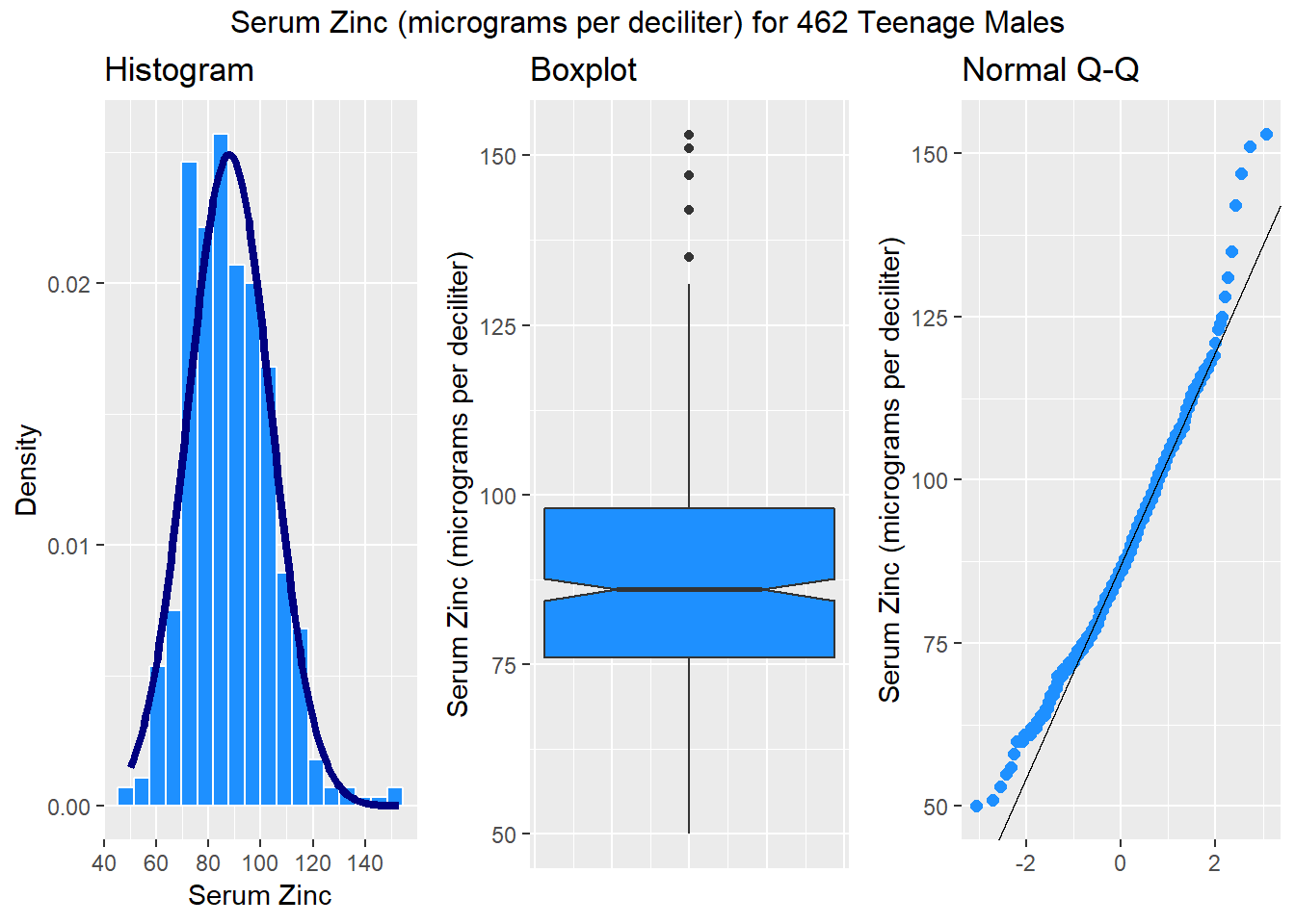
These results include some of the more useful plots and numerical summaries when assessing shape, center and spread. The zinc data in the serzinc data frame appear to be slightly right skewed, with five outlier values on the high end of the scale, in particular.
You could potentially add coord_flip() + to the histogram, and this would have the advantage of getting all three plots oriented in the same direction, but then we (or at least I) lose the ability to tell the direction of skew at a glance from the direction of the histogram.
16.3.3 Numerical Summaries
This section describes some numerical summaries of interest to augment the plots in summarizing the center, spread and shape of the distribution of serum zinc among these 462 teenage males.
The tables below are built using two functions from the Love-boost.R script.
skew1provides the skew1 value for thezincdata andEmp_Ruleprovides the results of applying the68-95-99.7Empirical Rule to thezincdata.
| min | Q1 | median | Q3 | max | mean | sd | n | missing |
|---|---|---|---|---|---|---|---|---|
| 50 | 76 | 86 | 98 | 153 | 87.94 | 16 | 462 | 0 |
[1] 0.121The skew1 value backs up our graphical assessment, that the data are slightly right skewed.
We can also assess how well the 68-95-99.7 Empirical Rule for a Normal distribution holds up for these data. Not too badly, as it turns out.
| count | proportion | |
|---|---|---|
| Mean +/- 1 SD | 323 | 0.6991 |
| Mean +/- 2 SD | 447 | 0.9675 |
| Mean +/- 3 SD | 458 | 0.9913 |
| Entire Data Set | 462 | 1 |
| vars | n | mean | sd | median | trimmed | mad | min | max | |
|---|---|---|---|---|---|---|---|---|---|
| X1 | 1 | 462 | 87.94 | 16 | 86 | 87.17 | 16.31 | 50 | 153 |
| range | skew | kurtosis | se | |
|---|---|---|---|---|
| X1 | 103 | 0.6191 | 0.8732 | 0.7446 |
Rounded to two decimal places, the standard deviation of the serum zinc data turns out to be 16, and so the standard error of the mean, shown as se in the psych::describe output, is 16 divided by the square root of the sample size, n = 462. This standard error is about to become quite important to us in building statistical inferences about the mean of the entire population of teenage males based on this sample.
References
Pagano, Marcello, and Kimberlee Gauvreau. 2000. Principles of Biostatistics. Second. Duxbury Press.
Reference values for those over the age of 10 years at http://www.mayomedicallaboratories.com/test-catalog/Clinical+and+Interpretive/8620 , visited 2017-08-17.↩