Chapter 36 Partial Review to help you prepare for Quiz 2
There are 15 items here, and then a set of answer sketches follow the questions. This isn’t a complete review - there are no questions here about either ANOVA or Mantel-Haenszel methods, for instance, and each might show up on Quiz 2.
36.1 Review Items 1-7
Researchers comparing the effectiveness of two pain medications randomly selected a group of patients who had been complaining of a certain kind of joint pain. They randomly divided those people into two groups, then administered the medications. Of the 85 people in the group who received medication A, 65 said that it provided relief. Of the 70 people in the group receiving medication B, 45 reported that it provided relief.
- Use the single augmentation with an imaginary failure or success (SAIFS) approach to specify a 95% confidence interval for the proportion of people who find relief from this kind of joint pain by using medication A.
- Now use the same approach to specify a 95% confidence interval for the proportion of people who find relief using medication B.
- Do the confidence intervals in items 1 and 2 overlap? What conclusions can you draw in light of that overlap (or lack thereof) about whether medication A or medication B is significantly more effective?
- Specify and display the correct 2x2 table (incorporating a Bayesian augmentation) analysis to enable you to study the A - B difference in the true proportions of people who find these medications effective.
- Use the 2x2 table results to specify an appropriate odds ratio and its 95% confidence interval in this situation, and explain what the values mean in context.
- Specify the hypotheses (H0 and HA) tested by the Fisher exact test you obtain in your 2x2 table. What does the provided p value tell you about what conclusion you should draw in this case regarding those hypotheses?
- If you have made an error in your conclusion for item 6, was it a Type I error or a Type II error? How do you know?
36.2 Review Items 8-9
For each of the following statements, indicate whether or not the statement is true or false, and specify how you know.
- If there is sufficient evidence to reject a null hypothesis at the 10% level, then there is sufficient evidence to reject it at the 5% level.
- A sample histogram will follow a normal distribution if the sample size is large enough.
36.3 Review Items 10-13
Charles Darwin carried out an experiment to study whether seedlings from cross-fertilized plants tend to be superior to those from self-fertilized plants. He covered a number of plants with fine netting so that insects would be unable to fertilize them. He fertilized a number of flowers on each plant with their own pollen and he fertilized an equal number of flowers on the same plant with pollen from a distant plant. (He did not specify how he decided which flowers received which treatments.) The seeds from the flowers were allowed to ripen and were set in wet sand to germinate. He placed two seedlings of the same age in a pot, one from a seed from a self-fertilized flower and one from a cross-fertilized flower.
He repeated this process with a total of 15 such pots. Each pot was then set aside for a time, so that the two plants in the plot would receive similar exposure to atmospheric conditions (sun, rainfall, etc.). Later, he gathered the heights of the plants (in inches) that came from those 15 cross-fertilized and 15 self-fertilized seeds at certain points in time. Those data are contained in the darwin.csv data set on our course website.
- Does this study call for a paired samples or independent samples comparison? How do you know?
- Display and interpret an appropriate graph to determine whether a t-test or a Wilcoxon test would be more appropriate for these data.
- Use the method (t or Wilcoxon) you specified in item 11 to find an appropriate 95% confidence interval for the average height difference between cross-fertilized and self-fertilized seedlings. Verify that your confidence interval describes the “cross” - “self” difference, rather than the opposite direction.
- Use an appropriate bootstrap procedure (setting your random seed to be
4310) to provide an alternative answer for the question posed in item 12. Is this bootstrap confidence interval wider or narrower than the interval you produced in item 12?
36.4 Review Items 14-15
You have been asked how large a sample size will be required for a clinical trial comparing two different approaches to blood pressure control. In approach A, we believe that the average systolic blood pressure will drop by 7 mm Hg, on the basis of our prior work in this area, while in the new approach B, we hope to see a clinically meaningful additional decline - specifically, we are looking for at least a 50% larger decline, so that the average systolic blood pressure will drop by 10.5 mm Hg or more over the same amount of time. Thus, the minimum clinically meaningful difference we are looking for is 3.5 mm Hg. Suppose we believe that the relevant standard deviation is 9 mm Hg, and we want to complete the trial using a 5% significance level and a two-sided t test.
- What will be the power of the test if we have a balanced design with 120 subjects in approach A and 120 different subjects in approach B? Show your calculation, and state your final result in a sentence.
- What is the smallest total sample size that we can use in a balanced design to maintain at least 90% power to detect the difference of interest, while still using independent samples? Show your calculation, and state your final result in a sentence.
36.5 Answer Sketch for Review Items
36.5.1 Answer 1
Sample Proportion             0.025             0.975
            0.765             0.663             0.859
The 95% confidence interval for the proportion of people using medication A who obtain relief is (0.663, 0.859). We are 95% confident that the true percentage of people who find relief using medication A is between 66.3% and 85.9%.
36.5.2 Answer 2
Sample Proportion             0.025             0.975
            0.643             0.519             0.762
The 95% confidence interval for the proportion of people using medication B who obtain relief is (0.519, 0.762).
36.5.3 Answer 3
The confidence intervals do overlap, so we cannot conclude from the separate intervals that there is (or isn’t) a statistically significant difference in the effectiveness rates for medications A and B. If the confidence intervals didn’t overlap, then we would know that there was a statistically significant difference in effectiveness between the two medications.
36.5.4 Answer 4
2 by 2 table analysis:
------------------------------------------------------
Outcome   : Relief
Comparing : Med. A vs. Med. B

       Relief No Relief    P(Relief) 95% conf. interval
Med. A     66        21        0.759     0.658    0.837
Med. B     46        26        0.639     0.522    0.741

                                  95% conf. interval
             Relative Risk:  1.19    0.9623    1.465
         Sample Odds Ratio:  1.78    0.8934    3.532
Conditional MLE Odds Ratio:  1.77    0.8446    3.749
    Probability difference:  0.12   -0.0223    0.259

             Exact P-value: 0.117
        Asymptotic P-value: 0.101
------------------------------------------------------
36.5.5 Answer 5
The odds ratio is 1.78, with 95% confidence interval (0.89, 3.53). The point estimate states that the odds of finding relief with medication A are 78% higher than the odds of finding relief with medication B. But the confidence interval indicates that, with 95% confidence, we can conclude only that the odds of relief with medication A are between 0.89 and 3.53 times as high as the odds of relief with medication B. Since 1 is in that confidence interval, we must conclude that there is no statistically significant effect of the medication choice on the odds of this outcome.
36.5.6 Answer 6
- H0: Medication Choice (A or B) is unrelated to the probability of Relief
- HA: Medication Choice and Relief are associated
The p value is 0.12, from the Fisher exact test. This means that we must retain the null hypothesis, and conclude that there is no significant association between Medication choice and the probability of Relief.
36.5.7 Answer 7
You would have made a Type II error. A Type II error can be made if you incorrectly retain H0. Since we retain H0, if we’ve made an error, it must have been a Type II error, since a Type I error occurs when you incorrectly reject H0.
36.5.8 Answer 8
This is FALSE. Sufficient evidence to reject H0 at the 10% level means that we have a p value < 0.10. In order to have sufficient evidence to reject H0 at the 5% level, we’d need to have a p value < 0.05. If our p < 0.10, this doesn’t guarantee that it is also true that p < 0.05.
36.5.9 Answer 9
Also FALSE. The mean of a sample will approach a Normal distribution, but if the data are skewed, the data will still be skewed no matter how many observations we see.
36.5.10 Answer 10
These samples are paired by the pot. Each pot provides a cross-fertilized seedling height and a self-fertilized seedling height. We should be comparing paired differences.
36.5.11 Answer 11
We need a plot of the 15 paired differences, for example a boxplot, or a normal Q-Q plot.
darwin$diffs <- darwin$cross.fertilized - darwin$self.fertilized

p1 <- ggplot(darwin, aes(x = diffs)) +
  geom_histogram(aes(y = ..density..), bins = fd_bins(darwin$diffs),
                 fill = "forestgreen", col = "white") +
  stat_function(fun = dnorm,
                args = list(mean = mean(darwin$diffs),
                            sd = sd(darwin$diffs)),
                lwd = 1.5, col = "navy") +
  labs(title = "Histogram",
       x = "Height Diff.", y = "Density")

p2 <- ggplot(darwin, aes(x = 1, y = diffs)) +
  geom_boxplot(fill = "forestgreen", outlier.color = "forestgreen") +
  theme(axis.text.x = element_blank(), axis.ticks.x = element_blank()) +
  labs(title = "Boxplot",
       y = "Difference in Seedling Height (inches)", x = "")

p3 <- ggplot(darwin, aes(sample = diffs)) +
  geom_qq(col = "forestgreen", size = 2) +
  geom_abline(intercept = qq_int(darwin$diffs),
              slope = qq_slope(darwin$diffs)) +
  labs(title = "Normal Q-Q",
       y = "Difference in Seedling Height (inches)", x = "")

gridExtra::grid.arrange(p1, p2, p3, nrow=1,
   top = "Cross-Self Fertilized Difference in Seedling Height
   in inches for 15 pairs of seedlings")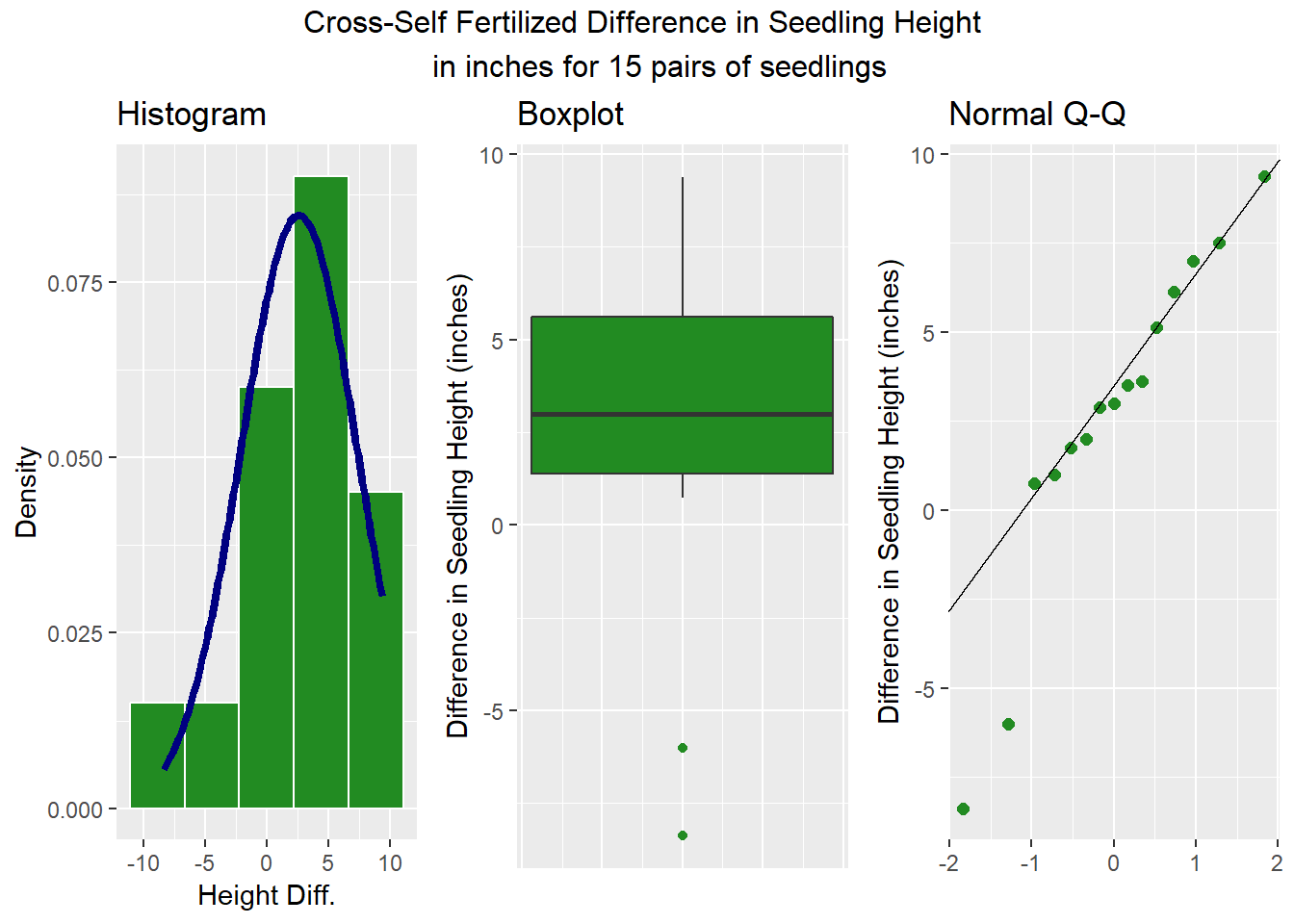
It appears that we have two low outliers out of the 15 paired differences. Assuming normality seems inappropriate here. I would probably use a Wilcoxon approach instead.
36.5.12 Answer 12
    Wilcoxon signed rank test

data:  darwin$diffs
V = 100, p-value = 0.04
alternative hypothesis: true location is not equal to 0
95 percent confidence interval:
 0.50 5.19
sample estimates:
(pseudo)median
          3.12
The cross-self differences appear to have a population pseudomedian which we are 95% confident is between 0.5 and 5.2 inches. The cross-fertilized plants appear to be statistically significantly taller on average than the self-fertilized plants in the same pot.
36.5.13 Answer 13
 Mean Lower Upper
2.617 0.208 4.734
This confidence interval is a bit narrower than the interval in item 12, and also shifted a bit closer to zero. We are 95% confident that the population mean cross-self difference is between 0.2 and 4.7 inches.
36.5.14 Answer 14
     Two-sample t test power calculation

              n = 120
          delta = 3.5
             sd = 9
      sig.level = 0.05
          power = 0.851
    alternative = two.sided

NOTE: n is number in *each* group
Such a test will have just over 85% power to detect the specified minimum clinically meaningful difference of 3.5 mm Hg, using a 5% two-sided significance level.
36.5.15 Answer 15
     Two-sample t test power calculation

              n = 140
          delta = 3.5
             sd = 9
      sig.level = 0.05
          power = 0.9
    alternative = two.sided

NOTE: n is number in *each* group
The minimum sample size we’ll need is 140 subjects in each approach (A and B), so that’s a total sample size of 280, to achieve 90% or higher power for the specified test while still using independent samples.