Chapter 24 Comparing Two Means Using Paired Samples
In this section, we apply several methods of testing the null hypothesis that two populations have the same distribution of a quantitative variable. In particular, we’ll focus on the comparison of means using paired sample t tests, signed rank tests, and bootstrap approaches. Our example comes from the Lead in the Blood of Children study, described in Section 17 and then developed further (including confidence intervals) in Section 20.
Recall that in that study, we measured blood lead content, in mg/dl, for 33 matched pairs of children, one of which was exposed (had a parent working in a battery factory) and the other of which was control (no parent in the battery factory, but matched to the exposed child by age, exposure to traffic and neighborhood). We then created a variable called leaddiff which contained the (exposed - control) differences within each pair.
# A tibble: 33 x 4
   pair  exposed control leaddiff
   <fct>   <int>   <int>    <int>
 1 P01        38      16       22
 2 P02        23      18        5
 3 P03        41      18       23
 4 P04        18      24       -6
 5 P05        37      19       18
 6 P06        36      11       25
 7 P07        23      10       13
 8 P08        62      15       47
 9 P09        31      16       15
10 P10        34      18       16
# ... with 23 more rows
24.1 Specifying A Two-Sample Study Design
These questions will help specify the details of the study design involved in any comparison of means.
- What is the outcome under study?
- What are the (in this case, two) treatment/exposure groups?
- Were the data collected using matched / paired samples or independent samples?
- Are the data a random sample from the population(s) of interest? Or is there at least a reasonable argument for generalizing from the sample to the population(s)?
- What is the significance level (or, the confidence level) we require here?
- Are we doing one-sided or two-sided testing/confidence interval generation?
- If we have paired samples, did pairing help reduce nuisance variation?
- If we have paired samples, what does the distribution of sample paired differences tell us about which inferential procedure to use?
- If we have independent samples, what does the distribution of each individual sample tell us about which inferential procedure to use?
24.1.1 For the bloodlead study
- The outcome is blood lead content in mg/dl.
- The groups are exposed (had a parent working in a battery factory) and control (no parent in the battery factory, but matched to the exposed child by age, exposure to traffic and neighborhood) children.
- The data were collected using matched samples. The pairs of subjects are matched by age, exposure to traffic and neighborhood.
- The data aren’t a random sample of the population of interest, but we will assume for now that there’s no serious issue with representing that population.
- We’ll use a 10% significance level (or 90% confidence level) in this setting.
- We’ll use a two-sided testing and confidence interval approach.
To answer question 7 (did pairing help reduce nuisance variation), we return to Section 17 where we saw that:
- The stronger the Pearson correlation coefficient, the more helpful pairing will be.
- Here, a straight line model using the control child’s blood lead content accounts for about 3% of the variation in blood lead content in the exposed child.
- So, as it turns out, pairing will have only a modest impact here on the inferences we draw in the study.
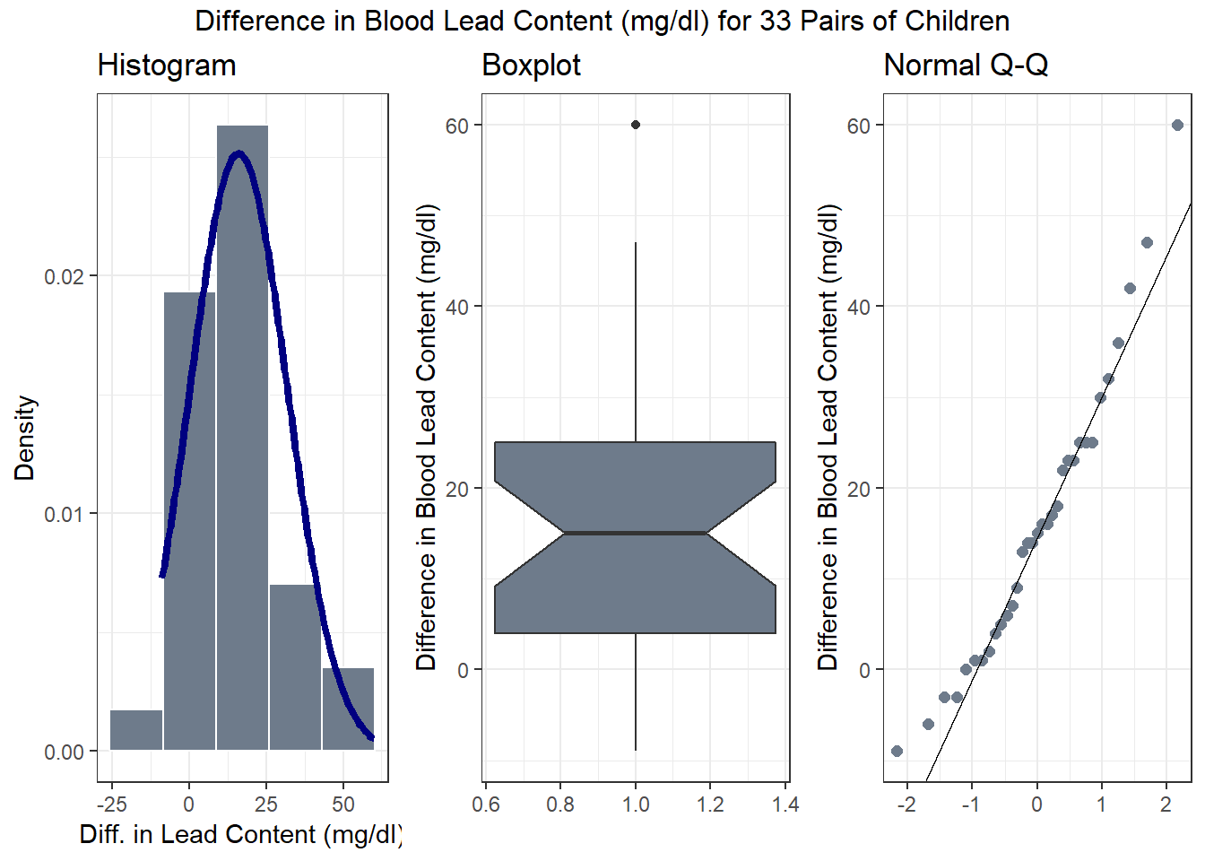
To address question 8, we’ll need to look at the data - specifically the paired differences. Repeating a panel of plots from Section 17, we will see that the paired differences appear to follow a Normal distribution, at least approximately (there’s a single outlier, but with 33 pairs, that’s not much of a concern, and the data are basically symmetric), so that a t-based procedure may be appropriate, or, at least, we’d expect to see similar results with t and bootstrap procedures.
Of course, question 9 doesn’t apply here, because we have paired, and not independent samples.
24.2 Hypothesis Testing for the Blood Lead Example
24.2.1 Our Research Question
Is there reasonable evidence, based on these paired samples of 33 exposed and 33 control children, for us to conclude that the population of children similar to those in the exposed group will have a distribution of blood lead content that is statistically significantly different from the population of children similar to those in the control group. In other words, if we generated the population of all exposed-control differences across the entire population of such pairs, would that distribution of paired differences be centered at zero (indicating no difference in the means)?
Again, the key idea is to calculate the paired differences (exposed - control, for example) in each pair, and then treat the result as if it were a single sample and apply the methods discussed in Section 22.
24.2.2 Specify the null hypothesis
Our null hypothesis here is that the population (true) mean blood lead content in the exposed group is the same as the population mean blood lead content in the control group plus a constant value (which we’ll symbolize with \(\Delta_0\) which is most often taken to be zero. Since we have paired samples, we can instead describe this hypothesis in terms of the difference between exposed and control within each pair. So, our null hypothesis can be written either as:
\[ H_0: \mu_{Exposed} = \mu_{Control} + \Delta_0 \] where \(\Delta_0\) is a constant, usually taken to be zero, or
\[ H_0: \mu_{Exposed - Control} = \Delta_0, \] where, again, \(\Delta_0\) is usually zero.
We will generally take this latter approach, where the population mean of the paired differences (here, exposed - control, but we could have just as easily selected control - exposed: the order is arbitrary so long as we are consistent) is compared to a constant value, usually 0.
For the bloodlead example, our population parameter \(\mu_{Exposed - Control}\) = the mean difference in blood lead content between the exposed and control groups (in mg/dl) across the entire population.
- We’re testing whether \(\mu\) is significantly different from a pre-specified value, 0 mg/dl.
24.2.3 Specify the research hypothesis
The research hypothesis is that the population mean of the exposed - control differences is not equal to our constant value \(\Delta_0\).
\[ H_A: \mu_{Exposed - Control} \neq \Delta_0, \]
For the bloodlead example, we have \(H_A: \mu_{Exposed - Control} \neq 0.\)
24.2.4 Specify the test procedure and \(\alpha\)
As we’ve seen in Section 20, there are several ways to build a confidence interval to address these hypotheses, and each of those approaches provides information about a related hypothesis test. This includes several methods for obtaining a paired t test, plus a Wilcoxon signed rank test, and a bootstrap comparison of means (or medians, etc.) using paired samples. We’ll specify an \(\alpha\) value of .10 here, indicating a 10% significance level (and 90% confidence level.)
24.2.5 Calculate the test statistic and \(p\) value
For the paired t test and Wilcoxon signed rank test, Section 20 demonstrated the relevant R code for the bloodlead example to obtain p values. For the bootstrap procedure, we again build a confidence interval. We repeat that work below.
24.2.6 Draw a conclusion
As we’ve seen, we use the \(p\) value to either
- reject \(H_0\) in favor of the alternative \(H_A\) (concluding that there is a statistically significant difference/association at the \(\alpha\) significance level) if the \(p\) value is less than our desired \(\alpha\) or
- retain \(H_0\) (and conclude that there is no statistically significant difference/association at the \(\alpha\) significance level) if the \(p\) value is greater than or equal to \(\alpha\).
24.3 Assuming a Normal distribution in the population of paired differences yields a paired t test.
    One Sample t-test

data:  bloodlead$exposed - bloodlead$control
t = 6, df = 30, p-value = 2e-06
alternative hypothesis: true mean is not equal to 0
90 percent confidence interval:
 11.3 20.6
sample estimates:
mean of x
       16
The t test statistic here is 6, based on 30 degrees of freedom, and this yields a p value of 2.036e-06 or 2.036 \(\times 10^{-6}\), or \(p\) = .000002036. This p value is certainly less than our pre-specified \(\alpha\) of 0.10, and so we’d reject \(H_0\) and conclude that the population mean of the exposed-control paired differences is statistically significantly different from 0.
- Notice that we would come to the same conclusion using the confidence interval. Specifically, using a 10% significance level (i.e. a 90% confidence level) a reasonable range for the true value of the population mean is entirely above 0 – it’s (11.3, 20.6). So if 0 is not in the 90% confidence interval, we’d reject \(H_0 : \mu_{Exposed - Control} = 0\) at the 10% significance level.
24.3.1 Assumptions of the paired t test
We must be willing to believe that
- the paired differences data are a random (or failing that, representative) sample from the population of interest, and
- that the samples were drawn independently, from an identical population distribution
regardless of what testing procedure we use. For the paired t test, we must also assume that:
- the paired differences come from a Normally distributed population.
24.3.2 Using broom to tidy the paired t test
# A tibble: 1 x 8
  estimate statistic p.value parameter conf.low conf.high method
     <dbl>     <dbl>   <dbl>     <dbl>    <dbl>     <dbl> <chr>
1     16.0      5.78 2.04e-6        32     11.3      20.6 One S~
# ... with 1 more variable: alternative <chr>
We can use the tidy function within the broom package to summarize the results of a t test, just as we did with a t-based confidence interval.
24.3.3 Calculation Details: The Paired t test
The paired t test is calculated using:
- \(\bar{d}\), the sample mean of the paired differences,
- the null hypothesized value \(\Delta_0\) for the differences (which is usually 0),
- \(s_d\), the sample standard deviation, and
- \(n\), the sample size (number of pairs).
We have
\[ t = \frac{\bar{d} - \Delta_0}{s_d/\sqrt{n}} \]
which is then compared to a \(t\) distribution with \(n - 1\) degrees of freedom to obtain a \(p\) value.
Wikipedia’s page on Student’s t test is a good resource for these calculations.
24.4 The Bootstrap Approach: Build a Confidence Interval
The same bootstrap approach is used for paired differences as for a single sample. We again use the smean.cl.boot() function in the Hmisc package to obtain bootstrap confidence intervals for the population mean, \(\mu_d\), of the paired differences in blood lead content.
set.seed(431888)
Hmisc::smean.cl.boot(bloodlead$exposed - bloodlead$control, conf.int = 0.90, B = 1000)
Mean Lower Upper
16.0 11.6 20.6 Since 0 is not contained in this 90% confidence interval, we reject the null hypothesis (that the mean of the paired differences in the population is zero) at the 10% significance level, so we know that p < 0.10.
24.4.1 Assumptions of the paired samples bootstrap procedure
We still must be willing to believe that
- the paired differences data are a random (or failing that, representative) sample from the population of interest, and
- that the samples were drawn independently, from an identical population distribution
regardless of what testing procedure we use. But, for the bootstrap, we do not also need to assume Normality of the population distribution of paired differences.
24.5 The Wilcoxon signed rank test (doesn’t require Normal assumption).
We could also use the Wilcoxon signed rank procedure to generate a CI for the pseudo-median of the paired differences.
    Wilcoxon signed rank test with continuity correction

data:  bloodlead$leaddiff
V = 500, p-value = 1e-05
alternative hypothesis: true location is not equal to 0
90 percent confidence interval:
 11.0 20.5
sample estimates:
(pseudo)median
          15.5
Using the Wilcoxon signed rank test, we obtain a two-sided p value of 1.155 \(\times 10^{-5}\), which is far less than our pre-specified \(\alpha\) of 0.10, so we would, again, reject \(H_0: \mu_{Exposed - Control} = 0\) at the 10% significance level.
- We can again use the
tidyfunction from thebroompackage to summarize the results of the Wilcoxon signed rank test.
# A tibble: 1 x 7
  estimate statistic  p.value conf.low conf.high method        alternative
     <dbl>     <dbl>    <dbl>    <dbl>     <dbl> <chr>         <chr>
1     15.5       499  1.15e-5     11.0      20.5 Wilcoxon sig~ two.sided
24.5.1 Assumptions of the Wilcoxon Signed Rank procedure
We still must be willing to believe that
- the paired differences data are a random (or failing that, representative) sample from the population of interest, and
- that the samples were drawn independently, from an identical population distribution
regardless of what testing procedure we use. But, for the Wilcoxon signed rank test, we also assume
- that the population distribution of the paired differences is symmetric, but potentially outlier-prone.
24.5.2 Calculation Details: The Wilcoxon Signed Rank test
- Calculate the paired difference for each pair, and drop those with difference = 0.
- Let N be the number of pairs, so there are 2N data points.
- Rank the pairs in order of smallest (rank = 1) to largest (rank = N) absolute difference.
- Calculate W, the sum of the signed ranks by \[ W = \sum_{i=1}^{N} [sgn(x_{2,i} - x_{1,i})] \prod R_i)]\]
- The sign function sgn(x) = -1 if x < 0, 0 if x = 0, and +1 if x > 0.
- Statistical software will convert W into a p value, given \(N\).
Wikipedia’s page on the Wilcoxon signed-rank test is a good resource for example calculations.
24.6 The Sign test
The sign test is something we’ve skipped in our discussion so far. It is a test for consistent differences between pairs of observations, just as the paired t test, Wilcoxon signed rank test and bootstrap for paired samples can provide. It has the advantage that it is relatively easy to calculate by hand, and that it doesn’t require the paired differences to follow a Normal distribution. In fact, it will even work if the data are substantially skewed.
- Calculate the paired difference for each pair, and drop those with difference = 0.
- Let \(N\) be the number of pairs that remain, so there are 2N data points.
- Let \(W\), the test statistic, be the number of pairs (out of N) in which the difference is positive.
- Assuming that \(H_0\) is true, then \(W\) follows a binomial distribution with probability 0.5 on \(N\) trials.
For example, consider our data on blood lead content:
 [1] 22  5 23 -6 18 25 13 47 15 16  6  1  2  7  0  4 -9 -3 36 25  1 16 42
[24] 30 25 23 32 17 9 -3 60 14 14| Difference | # of Pairs |
|---|---|
| Greater than zero | 28 |
| Equal to zero | 1 |
| Less than zero | 4 |
So we have \(N\) = 32 pairs, with \(W\) = 28 that are positive. We can calculate the p value using the binom.test approach in R:
    Exact binomial test

data:  28 and 32
number of successes = 30, number of trials = 30, p-value = 2e-05
alternative hypothesis: true probability of success is not equal to 0.5
95 percent confidence interval:
 0.710 0.965
sample estimates:
probability of success
0.875 - A one-tailed test can be obtained by substituting in “less” or “greater” as the alternative of interest.
- The confidence interval provided here doesn’t relate back to our original population means, of course. It’s just showing the confidence interval around the probability of the exposed mean being greater than the control mean for a pair of children.
24.7 Conclusions for the bloodlead study
Using any of these procedures, we would conclude that the null hypothesis (that the true mean of the paired differences is 0 mg/dl) is not tenable, and that it should be rejected at the 10% significance level. The smaller the p value, the stronger is the evidence that the null hypothesis is incorrect, and in this case, we have some fairly tiny p values.
| Procedure | p value | 90% CI for \(\mu_{Exposed - Control}\) | Conclusion |
|---|---|---|---|
| Paired t | \(2 \times 10^{-6}\) | 11.3, 20.6 | Reject \(H_0\). |
| Wilcoxon signed rank | \(1 \times 10^{-5}\) | 11, 20.5 | Reject \(H_0\). |
| Bootstrap CI | \(p\) < 0.10 | 11.6, 20.6 | Reject \(H_0\). |
| Sign test | \(2 \times 10^{-5}\) | None provided | Reject \(H_0\). |
Note that one-sided or one-tailed hypothesis testing procedures work the same way for paired samples as they did for single samples in Section 22.
24.8 Building a Decision Support Tool: Comparing Means
Are these paired or independent samples?
- If paired samples, then are the paired differences approximately Normally distributed?
- If yes, then a paired t test or confidence interval is likely the best choice.
- If no, is the main concern outliers (with generally symmetric data), or skew?
- If the paired differences appear to be generally symmetric but with substantial outliers, a Wilcoxon signed rank test is an appropriate choice, as is a bootstrap confidence interval for the population mean of the paired differences.
- If the paired differences appear to be seriously skewed, then we’ll usually build a bootstrap confidence interval, although a sign test is another reasonable possibility.