Chapter 25 Comparing Two Means Using Independent Samples

In this section, we apply several methods of testing the null hypothesis that two populations have the same distribution of a quantitative variable, based on independent samples of data. In particular, we’ll focus on the comparison of means using independent sample t tests, rank sum tests, and bootstrap approaches. Our example comes from the Ibuprofen in Sepsis trial, which was introduced in Section 18 and then further developed in Section 21

In that trial, 300 patients meeting specific criteria (including elevated temperature) for a diagnosis of sepsis were randomly assigned to either the Ibuprofen group (150 patients) and 150 to the Placebo group. Group information (our exposure) is contained in the treat variable. The key outcome of interest to us was temp_drop, the change in body temperature (in \(^{\circ}\)C) from baseline to 2 hours later, so that positive numbers indicate drops in temperature (a good outcome.)

sepsis %>% select(id, treat, temp_drop)

# A tibble: 300 x 3
   id    treat     temp_drop
   <chr> <fct>         <dbl>
 1 S002  Ibuprofen       1.4
 2 S004  Ibuprofen       0.4
 3 S005  Placebo         0  
 4 S006  Ibuprofen      -0.2
 5 S009  Ibuprofen       0.6
 6 S011  Ibuprofen      -0.4
 7 S012  Placebo        -0.1
 8 S014  Placebo         0.3
 9 S016  Placebo         0.1
10 S020  Ibuprofen       1.5
# ... with 290 more rows

25.1 Specifying A Two-Sample Study Design

Again, these questions will help specify the details of the study design involved in any comparison of means.

What is the outcome under study?
What are the (in this case, two) treatment/exposure groups?
Were the data collected using matched / paired samples or independent samples?
Are the data a random sample from the population(s) of interest? Or is there at least a reasonable argument for generalizing from the sample to the population(s)?
What is the significance level (or, the confidence level) we require here?
Are we doing one-sided or two-sided testing/confidence interval generation?
If we have paired samples, did pairing help reduce nuisance variation?
If we have paired samples, what does the distribution of sample paired differences tell us about which inferential procedure to use?
If we have independent samples, what does the distribution of each individual sample tell us about which inferential procedure to use?

25.1.1 For the `sepsis` study

The outcome is temp_drop, the change in body temperature (in \(^{\circ}\)C) from baseline to 2 hours later, so that positive numbers indicate drops in temperature (a good outcome.)
The groups are Ibuprofen and Placebo as contained in the treat variable in the sepsis tibble.
The data were collected using independent samples. The Ibuprofen subjects are not matched or linked to individual Placebo subjects - they are separate groups.
The subjects of the study aren’t drawn from a random sample of the population of interest, but they are randomly assigned to their respective treatments (Ibuprofen and Placebo) which will provide the reasoned basis for our inferences.
We’ll use a 10% significance level (or 90% confidence level) in this setting, as we did in our previous work on these data.
We’ll use a two-sided testing and confidence interval approach.

Questions 7 and 8 don’t apply, because these are independent samples of data, rather than paired samples.

To address question 9, we’ll need to look at the data in each sample. We’ll repeat the boxplot from Section 18, that allow us to assess the Normality of the distributions of (separately) the temp_drop results in the Ibuprofen and Placebo groups.

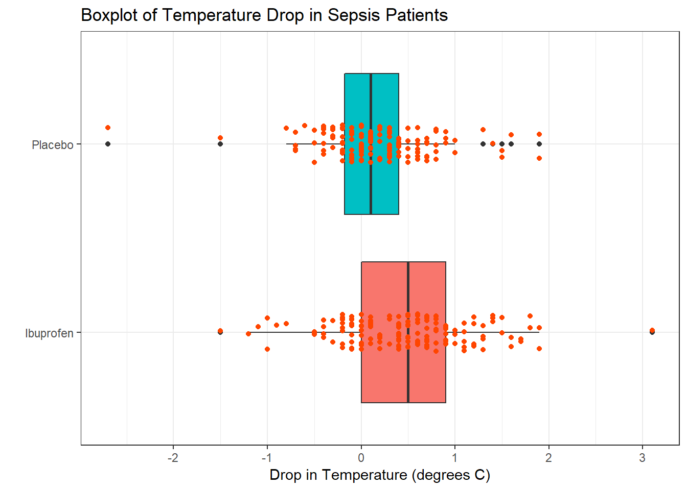
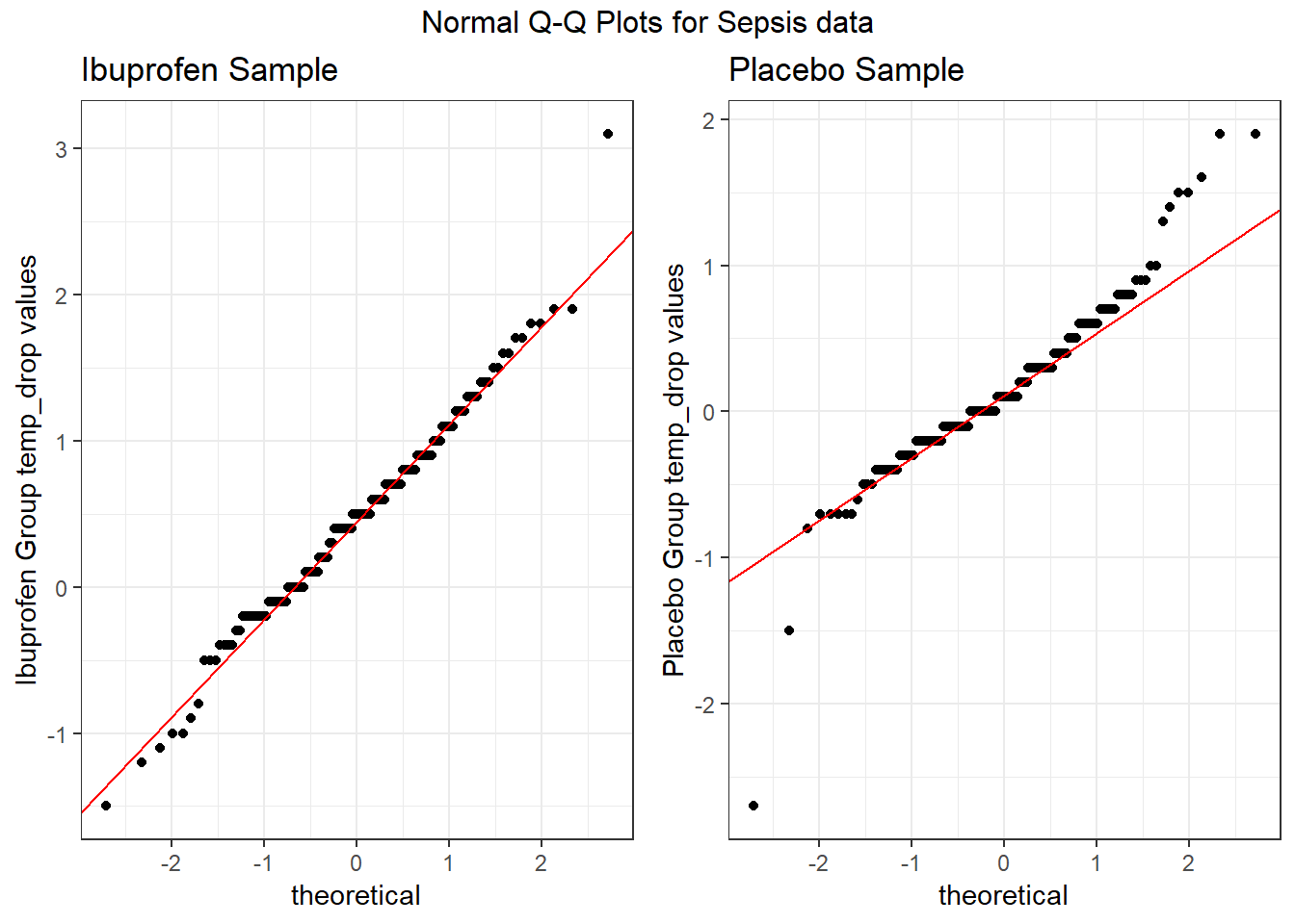
From these plots we conclude that the data in the Ibuprofen sample follow a reasonably Normal distribution, but this isn’t as true for the Placebo sample. It’s hard to know whether the apparent Placebo group outliers will affect whether the Normal distribution assumption is reasonable, but we’ll look into it.

25.2 Hypothesis Testing for the Sepsis Example

25.2.1 Our Research Question

Is there reasonable evidence, based on these samples of 150 Ibuprofen and 150 Placebo subjects, for us to conclude that those randomly assigned to receive Ibuprofen have a different population mean temp_drop than those randomly assigned to receive the Placebo? In other words, if we generated temp_drop results for Ibuprofen and Placebo at the population level, would the difference in (say) means be centered at zero, indicating no difference between the two treatments?

25.2.2 Specify the null hypothesis

Our null hypothesis here is that the population (true) mean temp_drop for subjects receiving Ibuprofen is the same as the population mean temp_drop for subjects receiving Placebo plus a constant value (which we’ll symbolize with \(\Delta_0\), which is again usually 0.) Since we have independent samples of data in this trial, we describe this hypothesis in terms of the difference between the separate population means. The hypotheses we are testing are:

\(H_0\): mean in population 1 = mean in population 2 + hypothesized difference \(\Delta_0\) vs.
\(H_A\): mean in population 1 \(\neq\) mean in population 2 + hypothesized difference \(\Delta_0\),

where \(\Delta_0\) is almost always zero. An equivalent way to write this is:

\(H_0: \mu_1 = \mu_2 + \Delta_0\) vs.
\(H_A: \mu_1 \neq \mu_2 + \Delta_0\)

Yet another equally valid way to write this is:

\(H_0: \mu_1 - \mu_2 = \Delta_0\) vs.
\(H_A: \mu_1 - \mu_2 \neq \Delta_0\),

where, again \(\Delta_0\) is almost always zero.

We will generally take this latter approach, where the difference in population means (here, we’ll use Ibuprofen - Placebo, but we could have just as easily selected Placebo - Ibuprofen: the order is arbitrary so long as we are consistent) is compared to a constant value, usually 0.

For the sepsis example, our population parameters \(\mu_{Ibuprofen}\) and \(\mu_{Placebo}\) are mean temperature drops (in \(^{\circ}\)C) from baseline to 2 hours later, so that positive numbers indicate drops in temperature (a good outcome.)

Our null hypothesis is that \(\mu_{Ibuprofen} - \mu{Placebo}\) is 0 degrees.

25.2.3 Specify the research hypothesis

The research hypothesis for the sepsis trial is that \(\mu_{Ibuprofen} - \mu{Placebo}\) is NOT 0 degrees.

25.2.4 Specify the test procedure and \(\alpha\)

As we’ve seen in Section 21, there are several ways to build a confidence interval to address these hypotheses, and each of those approaches provides information about a related hypothesis test. This includes the pooled t test, the Welch t test, the Wilcoxon-Mann-Whitney rank sum test, and a bootstrap comparison of means (or medians, etc.) using independent samples. We’ll specify an \(\alpha\) value of .10 here for the sepsis trial, indicating a 10% significance level (and 90% confidence level.)

25.2.5 Calculate the test statistic and \(p\) value

Section 21 demonstrated the relevant R code for the sepsis example to obtain p values. For the bootstrap procedure, we again build a confidence interval. We repeat that work below.

25.2.6 Draw a conclusion

As we’ve seen, we use the \(p\) value to either

reject \(H_0\) in favor of the alternative \(H_A\) (concluding that there is a statistically significant difference/association at the \(\alpha\) significance level) if the \(p\) value is less than our desired \(\alpha\) or
retain \(H_0\) (and conclude that there is no statistically significant difference/association at the \(\alpha\) significance level) if the \(p\) value is greater than or equal to \(\alpha\).

25.3 The Pooled T test

The standard method for comparing population means based on two independent samples is based on the t distribution, and requires the following assumptions:

[Independence] The samples for the two groups are drawn independently.
[Random Samples] The samples for each of the groups are drawn at random from the populations of interest.
[Normal Population] The two populations are each Normally distributed
[Equal Variances] The population variances in the two groups being compared are the same, so we can obtain a pooled estimate of their joint variance.

25.3.1 The Pooled t test Statistic

The test statistic is a t ratio, built up as follows.

\(t_{observed} = \frac{(\bar{x}_1 - \bar{x}_2) - \Delta_0}{SE_{pooled}(\bar{x}_1 - \bar{x}_2)}\),

where \(SE_{pooled}(\bar{x}_1 - \bar{x}_2)\) = \(\sqrt{\frac{s^2_{pooled}}{n_1} + \frac{s^2_{pooled}}{n_2}}\) and \(s^2_{pooled} = \frac{(n_1 - 1)s^2_1 + (n_2 - 1)s^2_2}{n_1 + n_2 - 2}\) and

where the p value is found by comparing this observed value \(t_{observed}\) to the t distribution with \(n_1 + n_2 - 2\) degrees of freedom.

25.3.2 The Pooled Variances t test in R

The pooled variances t test in R (also called the t test assuming equal population variances) is obtained as follows.

t.test(temp_drop ~ treat, data = sepsis, var.equal=TRUE)


    Two Sample t-test

data:  temp_drop by treat
t = 4, df = 300, p-value = 3e-05
alternative hypothesis: true difference in means is not equal to 0
95 percent confidence interval:
 0.168 0.455
sample estimates:
mean in group Ibuprofen   mean in group Placebo 
                  0.464                   0.153

We see from the t test output that the test statistic \(t_{observed} = 4.27\) is based on 298 degrees of freedom, which produces a p value of \(2.7 \times 10^{-5}\). This p value is much less than our chosen value for \(\alpha\) = 0.10, so we will clearly reject the null hypothesis and conclude that there is a statistically significant difference between the mean temperature drops in the Ibuprofen and Placebo groups.

25.3.3 Using `broom` to tidy the pooled t test

We can use the tidy function within the broom package to summarize the results of a t test, just as we did with a t-based confidence interval.

broom::tidy(t.test(temp_drop ~ treat, 
                   data = sepsis, var.equal=TRUE))

# A tibble: 1 x 9
  estimate1 estimate2 statistic p.value parameter conf.low conf.high method
      <dbl>     <dbl>     <dbl>   <dbl>     <dbl>    <dbl>     <dbl> <chr> 
1     0.464     0.153      4.27 2.68e-5       298    0.168     0.455 " Two~
# ... with 1 more variable: alternative <chr>

25.3.4 The Pooled T test in a Regression Model

Another way to obtain the pooled t test when comparing two population means using independent samples is to fit a simple regression model, that predicts the outcome of interest using an indicator variable to describe the exposure. For instance, in our sepsis trial, we have temp_drop as the outcome, and treat (Ibuprofen or Placebo) as the predictor in the following model.

sepsis.model1 <- lm(temp_drop ~ treat, data = sepsis)
summary(sepsis.model1)


Call:
lm(formula = temp_drop ~ treat, data = sepsis)

Residuals:
    Min      1Q  Median      3Q     Max 
-2.8527 -0.3640 -0.0527  0.3473  2.6360 

Coefficients:
             Estimate Std. Error t value Pr(>|t|)    
(Intercept)    0.4640     0.0516    8.99  < 2e-16 ***
treatPlacebo  -0.3113     0.0730   -4.27  2.7e-05 ***
---
Signif. codes:  0 '***' 0.001 '**' 0.01 '*' 0.05 '.' 0.1 ' ' 1

Residual standard error: 0.632 on 298 degrees of freedom
Multiple R-squared:  0.0575,    Adjusted R-squared:  0.0544 
F-statistic: 18.2 on 1 and 298 DF,  p-value: 2.68e-05

confint(sepsis.model1)

              2.5 % 97.5 %
(Intercept)   0.362  0.566
treatPlacebo -0.455 -0.168

The regression model estimates:

the point estimate for the population mean in the “Ibuprofen” group as 0.464
the estimated effect of “Placebo” as compared to “Ibuprofen” as -0.311
the p value from the pooled t test comparing “Ibuprofen” to “Placebo” as \(2.68 \times 10^{-5}\)
the 95% confidence interval associated with the pooled t test, of (-0.455, -0.168), which is just the negative of the result we obtained earlier (in this model, we are estimating Placebo - Ibuprofen, and in our t.test output, we estimated Ibuprofen - Placebo)

All of these values, drawn from the regression output above, match the pooled t test results.

25.4 The Welch T test

The default confidence interval based on the t test for independent samples in R uses something called the Welch test, in which the two populations being compared are not assumed to have the same variance. Each population is assumed to follow a Normal distribution, though, so the assumptions are:

[Independence] The samples for the two groups are drawn independently.
[Random Samples] The samples for each of the groups are drawn at random from the populations of interest.
[Normal Population] The two populations are each Normally distributed

It turns out that the Welch test gives essentially the same result as the pooled t test when either:

the design is balanced (our sample contains the same number of subjects in each group), or
the sample variances (equivalently, standard deviations) are quite similar in the two groups.

In our case, we have a balanced design, and so expect the Welch test and pooled t test to give nearly the same result.

25.4.1 The Welch t test in R

The Welch t test in R (also called the t test NOT assuming equal population variances) is obtained as follows.

t.test(temp_drop ~ treat, data = sepsis)


    Welch Two Sample t-test

data:  temp_drop by treat
t = 4, df = 300, p-value = 3e-05
alternative hypothesis: true difference in means is not equal to 0
95 percent confidence interval:
 0.168 0.455
sample estimates:
mean in group Ibuprofen   mean in group Placebo 
                  0.464                   0.153

We see from the t test output that the test statistic \(t_{observed} = 4.27\) is based on a fractional degrees of freedom, specifically 288.24 (this fractional df is characteristic of the Welch test) which produces a p value of \(2.7 \times 10^{-5}\). Again, since the p value is less than \(\alpha\) = 0.10, we will reject the null hypothesis and conclude that there is a statistically significant difference between the mean temperature drops in the Ibuprofen and Placebo groups.

25.4.2 Using `broom` to tidy the Welch t test

broom::tidy(t.test(temp_drop ~ treat, 
                   data = sepsis))

# A tibble: 1 x 10
  estimate estimate1 estimate2 statistic p.value parameter conf.low
     <dbl>     <dbl>     <dbl>     <dbl>   <dbl>     <dbl>    <dbl>
1    0.311     0.464     0.153      4.27 2.71e-5      288.    0.168
# ... with 3 more variables: conf.high <dbl>, method <chr>,
#   alternative <chr>

25.5 Bootstrap CI for \(\mu_1 - \mu_2\) from Independent Samples

As we saw in our plots earlier, assuming Normality, particularly in the Placebo population, is hard to justify. So we’ll consider methods that don’t require that assumption. The bootstrap approach to comparing population means using two independent samples still requires:

[Independence] The samples for the two groups are drawn independently.
[Random Samples] The samples for each of the groups are drawn at random from the populations of interest.

but does not require either of the other two assumptions.

25.5.1 Using the `bootdif` function from `Love-boost.R`

The bootdif function contained in the Love-boost.R script is a slightly edited version of the function at http://biostat.mc.vanderbilt.edu/wiki/Main/BootstrapMeansSoftware. Note that this approach uses a comma to separate the outcome variable (here, temp_drop) from the variable identifying the exposure groups (here, treat).

As in our previous bootstrap procedures, we are sampling (with replacement) a series of many data sets (default: 2000).

Here, we are building bootstrap samples based on the SBP levels in the two independent samples (Ibuprofen vs. Placebo).
For each bootstrap sample, we are calculating a mean difference between the two groups (Ibuprofen vs. Placebo).
We then determine the 5^th and 95^th percentile of the resulting distribution of mean differences (for a 90% confidence interval).

set.seed(431212)
bootdif(sepsis$temp_drop, sepsis$treat, conf.level = 0.90)

detach("package:Hmisc", unload=TRUE)

Mean Difference            0.05            0.95 
     -0.3113333      -0.4313333      -0.1973000

Since zero is not contained in this 90% confidence interval, we reject the null hypothesis (that the difference in population means between Ibuprofen and Placebo is zero) at the 10% significance level, so we know that p < 0.10.

Note: Running bootdif loads the Hmisc package which conflicts with some key functions in the tidyverse later. To remove these undesirable effects, I sometimes run detach("package:Hmisc", unload=TRUE) as above to try to help.

25.6 Wilcoxon-Mann-Whitney Rank Sum Test

The rank sum test is a non-parametric test of whether the two samples were selected from populations having the same distribution. The Wilcoxon-Mann-Whitney Rank Sum test still requires:

[Independence] The samples for the two groups are drawn independently.
[Random Samples] The samples for each of the groups are drawn at random from the populations of interest.

It also doesn’t really compare population means, so in that sense it can be a little confusing.

25.6.1 The Test Statistic

Assign numerical ranks to all observations across the two groups.
- 1 = smallest, n = largest. Use midpoint for any ties.
Add up the ranks from sample 1. Call that \(R_1\).
- \(R_2\) is then known, since the sum of all ranks is \(\frac{n(n+1)}{2}\)
\(U_1 = R_1 - \frac{n_1(n_1 + 1)}{2}\), where \(n_1\) is the sample size for sample 1.
\(U_1 + U_2\) is always just \(n_1 n_2\), so it doesn’t matter which sample you treat as sample 1.
The smaller of \(U_1\) and \(U_2\) is then called U, the test statistic.
Software converts U into a p value via a Normal approximation, given \(n_1\) and \(n_2\).

More details, including an alternative calculation approach, and a worked example are found on the Wikipedia page for the Mann-Whitney U test.

25.6.2 Wilcoxon-Mann-Whitney Rank Sum Test in R

wilcox.test(temp_drop ~ treat, data = sepsis, conf.int = TRUE)


    Wilcoxon rank sum test with continuity correction

data:  temp_drop by treat
W = 10000, p-value = 7e-06
alternative hypothesis: true location shift is not equal to 0
95 percent confidence interval:
 0.2 0.5
sample estimates:
difference in location 
                   0.3

25.7 The Continuity Correction

The p value for the rank sum test is obtained via a Normal approximation, using the test statistic W.

That approximation can be slightly improved through the use of a continuity correction (a small adjustment to account for the fact that we’re using a continuous distribution, the Normal, to approximate a discretely valued test statistic, W.)
The continuity correction is particularly important in the case where we have many tied ranks, and is applied by default in R.
If you want (for some reason) to not use it, add correct = FALSE to your call to the wilcox.test() function.

25.7.1 Tidying a Wilcoxon Rank Sum Test

broom::tidy(wilcox.test(temp_drop ~ treat, 
                 data = sepsis, conf.int = TRUE))

# A tibble: 1 x 7
  estimate statistic  p.value conf.low conf.high method        alternative
     <dbl>     <dbl>    <dbl>    <dbl>     <dbl> <chr>         <chr>      
1    0.300    14614.  7.28e-6    0.200     0.500 Wilcoxon ran~ two.sided

25.8 Conclusions for the `sepsis` study

Using any of these procedures, we would conclude that the null hypothesis (that the true difference between the Ibuprofen and Placebo mean temperature drops is 0 degrees) is untenable, and that it should be rejected at the 10% significance level. The smaller the p value, the stronger is the evidence that the null hypothesis is incorrect, and in this case, we have some fairly tiny p values.

The sample mean temperature drop for Ibuprofen was 0.464, and the sample mean for Placebo was 0.153.

Procedure	p value	90% CI for \(\mu_{Exposed - Control}\)	Conclusion
Pooled t test	\(2.7 \times 10^{-5}\)	0.168, 0.455	Reject \(H_0\).
Welch t test	\(2.7 \times 10^{-5}\)	0.168, 0.455	Reject \(H_0\).
Wilcoxon-Mann-Whitney rank sum test	\(7.3 \times 10^{-6}\)	0.2, 0.5	Reject \(H_0\).
Bootstrap CI from `bootdif`	p < 0.10	0.197, 0.431	Reject \(H_0\).

Note that one-sided or one-tailed hypothesis testing procedures work the same way for tests as they did for confidence intervals.

25.9 A More Complete Decision Support Tool: Comparing Means

Are these paired or independent samples?
If paired samples, then are the paired differences approximately Normally distributed?
1. If yes, then a paired t test or confidence interval is likely the best choice.
2. If no, is the main concern outliers (with generally symmetric data), or skew?
  1. If the paired differences appear to be generally symmetric but with substantial outliers, a Wilcoxon signed rank test is an appropriate choice, as is a bootstrap confidence interval for the population mean of the paired differences.
  2. If the paired differences appear to be seriously skewed, then we’ll usually build a bootstrap confidence interval, although a sign test is another reasonable possibility.
If independent, is each sample Normally distributed?
1. No –> use Wilcoxon-Mann-Whitney rank sum test or bootstrap via bootdif.
2. Yes –> are sample sizes equal?
  1. Balanced Design (equal sample sizes) - use pooled t test
  2. Unbalanced Design - use Welch test

25.10 Paired (Dependent) vs. Independent Samples

One area that consistently trips students up in this course is the thought process involved in distinguishing studies comparing means that should be analyzed using dependent (i.e. paired or matched) samples and those which should be analyzed using independent samples. A dependent samples analysis uses additional information about the sample to pair/match subjects receiving the various exposures. That additional information is not part of an independent samples analysis (unpaired testing situation.) The reasons to do this are to (a) increase statistical power, and/or (b) reduce the effect of confounding. Here are a few thoughts on the subject.

In the design of experiments, blocking is the term often used for the process of arranging subjects into groups (blocks) that are similar to one another. Typically, a blocking factor is a source of variability that is not of primary interest to the researcher An example of a blocking factor might be the sex of a patient; by blocking on sex, this source of variability is controlled for, thus leading to greater accuracy.

If the sample sizes are not balanced (not equal), the samples must be treated as independent, since there would be no way to precisely link all subjects. So, if we have 10 subjects receiving exposure A and 12 subjects receiving exposure B, a dependent samples analysis (such as a paired t test) is not correct.
The key element is a meaningful link between each observation in one exposure group and a specific observation in the other exposure group. Given a balanced design, the most common strategy indicating dependent samples involves two or more repeated measures on the same subjects. For example, if we are comparing outcomes before and after the application of an exposure, and we have, say, 20 subjects who provide us data both before and after the exposure, then the comparison of results before and after exposure should use a dependent samples analysis. The link between the subjects is the subject itself - each exposed subject serves as its own control.
The second most common strategy indicating dependent samples involves deliberate matching of subjects receiving the two exposures. A matched set of observations (often a pair, but it could be a trio or quartet, etc.) is determined using baseline information and then (if a pair is involved) one subject receives exposure A while the other member of the pair receives exposure B, so that by calculating the paired difference, we learn about the effect of the exposure, while controlling for the variables made similar across the two subjects by the matching process.
In order for a dependent samples analysis to be used, we need (a) a link between each observation across the exposure groups based on the way the data were collected, and (b) a consistent measure (with the same units of measurement) so that paired differences can be calculated and interpreted sensibly.
If the samples are collected to facilitate a dependent samples analysis, the correlation of the outcome measurements across the groups will often be moderately strong and positive. If that’s the case, then the use of a dependent samples analysis will reduce the effect of baseline differences between the exposure groups, and thus provide a more precise estimate. But even if the correlation is quite small, a dependent samples analysis should provide a more powerful estimate of the impact of the exposure on the outcome than would an independent samples analysis with the same number of observations.

25.10.1 Three “Tricky” Examples

Suppose we take a convenient sample of 200 patients from the population of patients who complete a blood test in April 2017 including a check of triglycerides, and who have a triglyceride level in the high category (200 to 499 mg/dl). Next, we select a patient at random from this group of 200 patients, and then identify another patient from the group of 200 who is the same age (to within 2 years) and also the same sex. We then randomly assign our intervention to one of these two patients and usual care without our intervention to the other patient. We then set these two patients aside and return to our original sample, repeating the process until we cannot find any more patients in the same age range and of the same gender. This generates a total of 77 patients who receive the intervention and 77 who do not. If we are trying to assess the effect of our intervention on triglyceride level in October 2017 using this sample of 154 people, should we use dependent (paired) or independent samples?
Suppose we take a convenient sample of 77 patients from the population of patients who complete a blood test in April 2017 including a check of triglycerides, and who have a triglyceride level in the high category (200 to 499 mg/dl). Next, we take a convenient sample of 77 patients from the population of patients who complete a blood test in May 2017 including a check of triglycerides, and who have a triglyceride level in the high category (200 to 499 mg/dl). We flip a coin to determine whether the intervention will be given to each of the 77 patients from April 2017 (if the coin comes up “HEADS”) or instead to each of the 77 patients from May 2017 (if the coin comes up “TAILS”). Then, we assign our intervention to the patients seen in the month specified by the coin and assign usual care without our intervention to the patients seen in the other month. If we are trying to assess the effect of our intervention on triglyceride level in October 2017 using this sample of 154 people, should we use dependent (paired) or independent samples?
Suppose we take a convenient sample of 200 patients from the population of patients who complete a blood test in April 2017 including a check of triglycerides, and who have a triglyceride level in the high category (200 to 499 mg/dl). For each patient, we re-measure them again in October 2017, again checking their triglyceride level. But in between, we take the first 77 of the patients in a randomly sorted list and assign them to our intervention (which takes place from June through September 2017) and take an additional group of 77 patients from the remaining part of the list and assign them to usual care without our intervention over the same time period. If we are trying to assess the effect of our intervention on each individual’s change in triglyceride level (from April/May to October) using this sample of 154 people, should we use dependent (paired) or independent samples?

25.10.2 Answers for the Three “Tricky” Examples

Answer for 1. Our first task is to identify the outcome and the exposure groups. Here, we are comparing the distribution of our outcome (triglyceride level in October) across two exposures: (a) receiving the intervention and (b) not receiving the intervention. We have a sample of 77 patients receiving the intervention, and a different sample of 77 patients receiving usual care. Each of the 77 subjects receiving the intervention is matched (on age and sex) to a specific subject not receiving the intervention. So, we can calculate paired differences by taking the triglyceride level for the exposed member of each pair and subtracting the triglyceride level for the usual care member of that same pair. Thus our comparison of the exposure groups should be accomplished using a dependent samples analysis, such as a paired t test.

Answer for 2. Again, we begin by identfying the outcome (triglyceride level in October) and the exposure groups. Here, we compare two exposures: (a) receiving the intervention and (b) receiving usual care. We have a sample of 77 patients receiving the intervention, and a different sample of 77 patients receiving usual care. But there is no pairing or matching involved. There is no connection implied by the way that the data were collected that implies that, for example, patient 1 in the intervention group is linked to any particular subject in the usual care group. So we need to analyze the data using independent samples.

Answer for 3. Once again, we identfy the outcome (now it is the within-subject change in triglyceride level from April to October) and the exposure groups. Here again, we compare two exposures: (a) receiving the intervention and (b) receiving usual care. We have a sample of 77 patients receiving the intervention, and a different sample of 77 patients receiving usual care. But again, there is no pairing or matching between the patients receiving the intervention and the patients receiving usual care. While each outcome value is a difference (or change) in triglyceride levels, there’s no connection implied by the way that the data were collected that implies that, for example, patient 1 in the intervention group is linked to any particular subject in the usual care group. So, again, we need to analyze the data using independent samples.

For more background and fundamental material, you might consider the Wikipedia pages on Paired Difference Test and on Blocking (statistics).