Chapter 46 Species Found on the Galapagos Islands

46.1 A Little Background

The gala data describe describe features of the 30 Galapagos Islands.

The Galapagos Islands are found about 900 km west of South America: specifically the continental part of Ecuador. The Islands form a province of Ecuador and serve as a national park and marine reserve. They are noted for their vast numbers of unique (or endemic) species and were studied by Charles Darwin during the voyage of the Beagle. I didn’t know most of this, but it’s on Wikipedia, so I’ll assume it’s all true until someone sets me straight.

galapic.jpg

46.1.1 Sources

The data were initially presented by Johnson M and Raven P (1973) Species number and endemism: the Galapagos Archipelago revisited. Science 179: 893-895 and also appear in several regression texts, including my source: Faraway (2015). Note that Faraway filled in some missing data to simplify things a bit. A similar version of the data is available as part of the faraway library in R, but I encourage you to use the version I supply on our web site.

46.1.2 Variables in the `gala` data frame

id = island identification code
island = island name
species = our outcome, the number of species found on the island
area = the area of the island, in square kilometers
elevation = the highest elevation of the island, in meters
nearest = the distance from the nearest island, in kilometers
scruz = the distance from Santa Cruz Island, in kilometers. Santa Cruz is the home to the largest human population in the Islands, and to the town of Puerto Ayora.
adjacent = the area of the adjacent island, in square kilometers

gala

# A tibble: 30 x 8
      id island       species  area elevation nearest scruz adjacent
   <int> <fct>          <int> <dbl>     <int>   <dbl> <dbl>    <dbl>
 1     1 Baltra            58 25.1        346     0.6   0.6     1.84
 2     2 Bartolome         31  1.24       109     0.6  26.3   572.  
 3     3 Caldwell           3  0.21       114     2.8  58.7     0.78
 4     4 Champion          25  0.1         46     1.9  47.4     0.18
 5     5 Coamano            2  0.05        77     1.9   1.9   904.  
 6     6 Daphne.Major      18  0.34       119     8     8       1.84
 7     7 Daphne.Minor      24  0.08        93     6    12       0.34
 8     8 Darwin            10  2.33       168    34.1 290.      2.85
 9     9 Eden               8  0.03        71     0.4   0.4    18.0 
10    10 Enderby            2  0.18       112     2.6  50.2     0.1 
# ... with 20 more rows

Hmisc::describe(gala) # check for missing and inexplicable values

gala 

 8  Variables      30  Observations
---------------------------------------------------------------------------
id 
       n  missing distinct     Info     Mean      Gmd      .05      .10 
      30        0       30        1     15.5    10.33     2.45     3.90 
     .25      .50      .75      .90      .95 
    8.25    15.50    22.75    27.10    28.55 

lowest :  1  2  3  4  5, highest: 26 27 28 29 30
---------------------------------------------------------------------------
island 
       n  missing distinct 
      30        0       30 

lowest : Baltra     Bartolome  Caldwell   Champion   Coamano   
highest: SantaFe    SantaMaria Seymour    Tortuga    Wolf      
---------------------------------------------------------------------------
species 
       n  missing distinct     Info     Mean      Gmd      .05      .10 
      30        0       27    0.999    85.23    109.5      2.0      2.9 
     .25      .50      .75      .90      .95 
    13.0     42.0     96.0    280.5    319.1 

lowest :   2   3   5   8  10, highest: 237 280 285 347 444
---------------------------------------------------------------------------
area 
       n  missing distinct     Info     Mean      Gmd      .05      .10 
      30        0       29        1    261.7    478.6   0.0390   0.0770 
     .25      .50      .75      .90      .95 
  0.2575   2.5900  59.2375 578.5460 782.6215 
                                                                      
Value          0    20    30    60   130   170   550   570   630   900
Frequency     17     3     1     2     1     1     1     1     1     1
Proportion 0.567 0.100 0.033 0.067 0.033 0.033 0.033 0.033 0.033 0.033
                
Value       4670
Frequency      1
Proportion 0.033
---------------------------------------------------------------------------
elevation 
       n  missing distinct     Info     Mean      Gmd      .05      .10 
      30        0       30        1      368    411.1    47.35    68.80 
     .25      .50      .75      .90      .95 
   97.75   192.00   435.25   868.20  1229.40 

lowest :   25   46   49   71   76, highest:  777  864  906 1494 1707
---------------------------------------------------------------------------
nearest 
       n  missing distinct     Info     Mean      Gmd      .05      .10 
      30        0       22    0.997    10.06    13.73    0.445    0.590 
     .25      .50      .75      .90      .95 
   0.800    3.050   10.025   34.100   40.205 

lowest :  0.2  0.4  0.5  0.6  0.7, highest: 16.5 29.1 34.1 45.2 47.4
---------------------------------------------------------------------------
scruz 
       n  missing distinct     Info     Mean      Gmd      .05      .10 
      30        0       29        1    56.98    65.17     0.49     0.60 
     .25      .50      .75      .90      .95 
   11.02    46.65    81.08    97.73   193.90 

lowest :   0.0   0.4   0.6   1.9   8.0, highest:  93.1  95.3 119.6 254.7 290.2
---------------------------------------------------------------------------
adjacent 
       n  missing distinct     Info     Mean      Gmd      .05      .10 
      30        0       21    0.998    261.1    477.8     0.10     0.10 
     .25      .50      .75      .90      .95 
    0.52     2.59    59.24   578.55   782.62 
                                                                
Value          0    20    30    60   130   570   630   900  4670
Frequency     17     2     2     2     2     2     1     1     1
Proportion 0.567 0.067 0.067 0.067 0.067 0.067 0.033 0.033 0.033
---------------------------------------------------------------------------

46.2 DTDP: A Scatterplot Matrix

After missingness and range checks, the first step in any data analysis problem is to draw the picture. The most useful picture for me in thinking about a regression problem with a reasonably small number of predictors is a scatterplot matrix.

Our outcome, that we are predicting here is the number of species.

We’ll use five predictors:

area
elevation
nearest
scruz and
adjacent.

pairs (~ species + area + elevation + nearest + scruz + adjacent,
       data=gala, main="Galapagos Islands Matrix", 
       upper.panel = panel.smooth,
       diag.panel = panel.hist,
       lower.panel = panel.cor)

46.2.1 Questions about the Scatterplot Matrix

What are we looking for in the scatterplots in the top row?
What can we learn from the Pearson correlations in the left column?
How do the histograms help increase our understanding of the data?
What about the scatterplots that are not in the top row?
What can we learn from the Pearson correlations that compare predictors?

46.3 Fitting A “Kitchen Sink” Linear Regression model

Next, we’ll fit a multiple linear regression model to predict the number of species based on the five predictors included in the gala data frame (and scatterplot matrix above.) We use the lm command to fit the linear model, and use what is called Wilkinson-Rogers notation to specify the model.

model1 <- lm(species ~ area + elevation + nearest + scruz + 
               adjacent, data=gala)
summary(model1)


Call:
lm(formula = species ~ area + elevation + nearest + scruz + adjacent, 
    data = gala)

Residuals:
    Min      1Q  Median      3Q     Max 
-111.68  -34.90   -7.86   33.46  182.58 

Coefficients:
            Estimate Std. Error t value Pr(>|t|)    
(Intercept)  7.06822   19.15420    0.37   0.7154    
area        -0.02394    0.02242   -1.07   0.2963    
elevation    0.31946    0.05366    5.95  3.8e-06 ***
nearest      0.00914    1.05414    0.01   0.9932    
scruz       -0.24052    0.21540   -1.12   0.2752    
adjacent    -0.07480    0.01770   -4.23   0.0003 ***
---
Signif. codes:  0 '***' 0.001 '**' 0.01 '*' 0.05 '.' 0.1 ' ' 1

Residual standard error: 61 on 24 degrees of freedom
Multiple R-squared:  0.766, Adjusted R-squared:  0.717 
F-statistic: 15.7 on 5 and 24 DF,  p-value: 6.84e-07

46.3.1 Questions about the Kitchen Sink Model Summaries

What conclusions can we draw from the summary output for this model? Specifically …

What is being predicted? What is the prediction equation?
How do we interpret the elevation estimate of 0.32?
How do we interpret the area estimate of -0.02?
How do we interpret the intercept estimate of 7.07?
Overall, does the model add statistically significant predictive value over the simplest possible model, using the intercept term alone?
What proportion of the variation in species counts does this model account for?
What does the residual standard error mean in this context?
What can we learn from the standard errors in the coefficient output?
What can we learn from the t values and Pr(>|t|) values in the coefficient output?
How should we interpret the meaning of the Adjusted R-squared value?

46.4 Finding Confidence Intervals for our Coefficient Estimates

confint(model1, level = 0.95)

               2.5 %  97.5 %
(Intercept) -32.4641 46.6005
area         -0.0702  0.0223
elevation     0.2087  0.4302
nearest      -2.1665  2.1848
scruz        -0.6851  0.2040
adjacent     -0.1113 -0.0383

46.4.1 Questions about the Confidence Intervals

What can we learn from the provided confidence interval for elevation?
How do the confidence interval results here compare to the t tests in the summary output?

46.5 Measuring Collinearity - the Variance Inflation Factor

The variance inflation factor (abbreviated VIF) can be used to quantify the impact of multicollinearity in a linear regression model.

The VIF is sometimes interpreted by taking its square root, and then interpreting the result as telling you how much larger the standard error for that coefficient is, as compared to what it would be if that variable were uncorrelated with the other predictors.

In R, the vif function from the car library, when applied to a linear regression model, specifies the variance inflation factors for each of the model’s coefficients, as follows.

vif(model1)

     area elevation   nearest     scruz  adjacent 
     2.93      3.99      1.77      1.68      1.83

So, for instance, the VIF of 3.99 for elevation implies that the standard error of the elevation coefficient is approximately 2 times larger than it would be if elevation was uncorrelated with the other predictors.

I will look closely at any VIF value that is greater than 5, although some people use a cutoff of 10.

Another collinearity measure called tolerance is simply 1/VIF.
For example, the tolerance for elevation would be 0.25, and the cutoff for a potentially problematic tolerance is either 0.2 or lower, or 0.1 or lower.

To calculate the VIF for a predictor \(x_1\), use all of the other predictors to predict \(x_1\) and find the multiple R² value.

VIF for \(x_1\) = 1 / (1 - \(R^2_{x_1 | others}\)), and tolerance = (1 - \(R^2_{x_1 | others}\)).

46.6 Global (F) Testing of Overall Significance

Our Galapagos Islands species count regression model (called model1) predicts the count of an island’s species using area, elevation, nearest, scruz and adjacent.

nullmodel <- lm(species ~ 1, data=gala)
summary(nullmodel)


Call:
lm(formula = species ~ 1, data = gala)

Residuals:
   Min     1Q Median     3Q    Max 
 -83.2  -72.2  -43.2   10.8  358.8 

Coefficients:
            Estimate Std. Error t value Pr(>|t|)    
(Intercept)     85.2       20.9    4.07  0.00033 ***
---
Signif. codes:  0 '***' 0.001 '**' 0.01 '*' 0.05 '.' 0.1 ' ' 1

Residual standard error: 115 on 29 degrees of freedom

anova(model1, nullmodel)

Analysis of Variance Table

Model 1: species ~ area + elevation + nearest + scruz + adjacent
Model 2: species ~ 1
  Res.Df    RSS Df Sum of Sq    F  Pr(>F)    
1     24  89231                              
2     29 381081 -5   -291850 15.7 6.8e-07 ***
---
Signif. codes:  0 '***' 0.001 '**' 0.01 '*' 0.05 '.' 0.1 ' ' 1

46.6.1 Questions about the Global Test via ANOVA

How do we interpret the null model fit above?
What are the hypotheses being tested by this ANOVA output?
What conclusions can we draw from the ANOVA output presented here?
Where do we find information regarding the result for the previous question in the summary output for the linear model?
How would we set up an ANOVA model to test whether the “kitchen sink” model’s predictive value would be significantly impacted by removing the adjacent predictor from the model?
Where do we find information regarding these result for the previous question in the summary output for the linear model?
How would we set an ANOVA model to test whether a model with area only would be a significant improvement over the null model?

46.7 Sequential Testing in a Regression Model with ANOVA

anova(model1)

Analysis of Variance Table

Response: species
          Df Sum Sq Mean Sq F value  Pr(>F)    
area       1 145470  145470   39.13 1.8e-06 ***
elevation  1  65664   65664   17.66 0.00032 ***
nearest    1     29      29    0.01 0.93007    
scruz      1  14280   14280    3.84 0.06173 .  
adjacent   1  66406   66406   17.86 0.00030 ***
Residuals 24  89231    3718                    
---
Signif. codes:  0 '***' 0.001 '**' 0.01 '*' 0.05 '.' 0.1 ' ' 1

46.7.1 Questions about Sequential Testing and ANOVA

What conclusions can we draw from the area row in the output above?
What conclusions can we draw from the elevation row?
Does nearest add statistically significant predictive value to the model including area and elevation, but none of the other predictors?
Does adjacent add significant predictive value as last predictor into the model?
Where else in the regression output can we find the answer to the previous question?
How does the mean square of the residuals (3718) relate to the residual standard error?
What percentage of the variation in the species counts is accounted for by area alone?
What percentage of the variation explained by the kitchen sink model would also be accounted for in a two-predictor regression model including area and elevation alone?
How could we use the original linear model output to whether a model using the four predictors that appear most promising here would be statistically significantly worse than the full model with all five predictors?
What does the following output do differently than the output above, and why is that potentially useful here? Why is the p value for scruz so different?

anova(lm(species ~ area + elevation + adjacent + scruz + nearest, data=gala))

Analysis of Variance Table

Response: species
          Df Sum Sq Mean Sq F value  Pr(>F)    
area       1 145470  145470   39.13 1.8e-06 ***
elevation  1  65664   65664   17.66 0.00032 ***
adjacent   1  73171   73171   19.68 0.00017 ***
scruz      1   7544    7544    2.03 0.16719    
nearest    1      0       0    0.00 0.99315    
Residuals 24  89231    3718                    
---
Signif. codes:  0 '***' 0.001 '**' 0.01 '*' 0.05 '.' 0.1 ' ' 1

Consider the ANOVA below, run on a new model with elevation after adjacent. What happens? Why?

anova(lm(species ~ area + adjacent + elevation + scruz + nearest, data=gala))

Analysis of Variance Table

Response: species
          Df Sum Sq Mean Sq F value  Pr(>F)    
area       1 145470  145470   39.13 1.8e-06 ***
adjacent   1   2850    2850    0.77    0.39    
elevation  1 135985  135985   36.58 3.0e-06 ***
scruz      1   7544    7544    2.03    0.17    
nearest    1      0       0    0.00    0.99    
Residuals 24  89231    3718                    
---
Signif. codes:  0 '***' 0.001 '**' 0.01 '*' 0.05 '.' 0.1 ' ' 1

46.8 An ANOVA table for the Model as a Whole

It’s probably also worthwhile to compute a completed ANOVA table for the model as a whole. All elements are in the ANOVA tables above, or the model summary.

Group	DF	SS	MS	F	P
Regression	5	291849	58369.8	15.7	6.838e-07
Residuals	24	89231	3718.0
Total	29	381080

How did I determine the Mean Square for the Regression model?
What conclusions can we draw from this ANOVA table?

46.9 Assumption Checking for our Galápagos Islands models

Remember that the key assumptions of multiple linear regression are:

[Linearity] We have also assumed that the structural part of the model is correctly specified (we’ve included all the predictors that need to be in the model, and expressed them in the most appropriate manner, and we’ve left out any predictors that don’t need to be in the model.)
[Normality] The regression makes errors that come from a Normal distribution
[Homoscedasticity = Constant Variance] The regression makes errors that come from a distribution with constant variance at all predictor levels.
[Independence] The regression errors are independent of each other.

In addition, we need to realize that sometimes a few observations may be particularly problematic. For instance:

An observation may simply not fit the model well (i.e. it creates a large residual)
An observation may have high leverage over the fit of the model (this happens with observations that have an unusual combination of predictor values, in particular)
An observation may actually have high influence on the model (in the sense that whether they are included or excluded has a large impact on the model’s fit, and the value of its parameter estimates.)
Or any combination of high residual, leverage and influence may occur.

So it is important to check the assumptions that we can with the data we have. Our most important tools are plots and other summaries of residuals, and what are called influence statistics.

46.10 My First Plot: Studentized Residuals vs. Fitted Values

The first diagnostic plot I usually draw for a multiple regression is a scatterplot of the model’s studentized residuals (on the vertical axis) vs. the model’s fitted values (on the horizontal.) This plot can be used to assess potential non-linearity, non-constant variance, and non-Normality in the residuals.

gala$stures <- rstudent(model1); gala$fits <- fitted(model1)
ggplot(gala, aes(x = fits, y = stures)) +
    theme_bw() + geom_point(size = 3, shape = 1) +
    geom_smooth(col = "blue", se = FALSE, weight = 0.5) +
    geom_hline(aes(yintercept = 0), linetype = "dashed") +
    labs(x = "Fitted Values of Species", 
         y = "Studentized Residuals",
         title = "gala data: Model 1\nStudentized Residuals vs. Fitted Values")

`geom_smooth()` using method = 'loess' and formula 'y ~ x'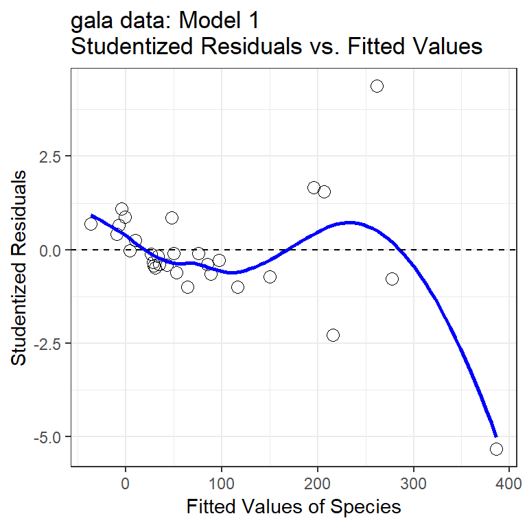

46.10.1 Questions about Studentized Residuals vs. Fitted Values

Consider the point at bottom right. What can you infer about this observation?
Why did I include the dotted horizontal line at Studentized Residual = 0?
What is the purpose of the thin blue line?
What does this plot suggest about the potential for outliers in the residuals?

46.11 Automatic Regression Diagnostics for Model 1

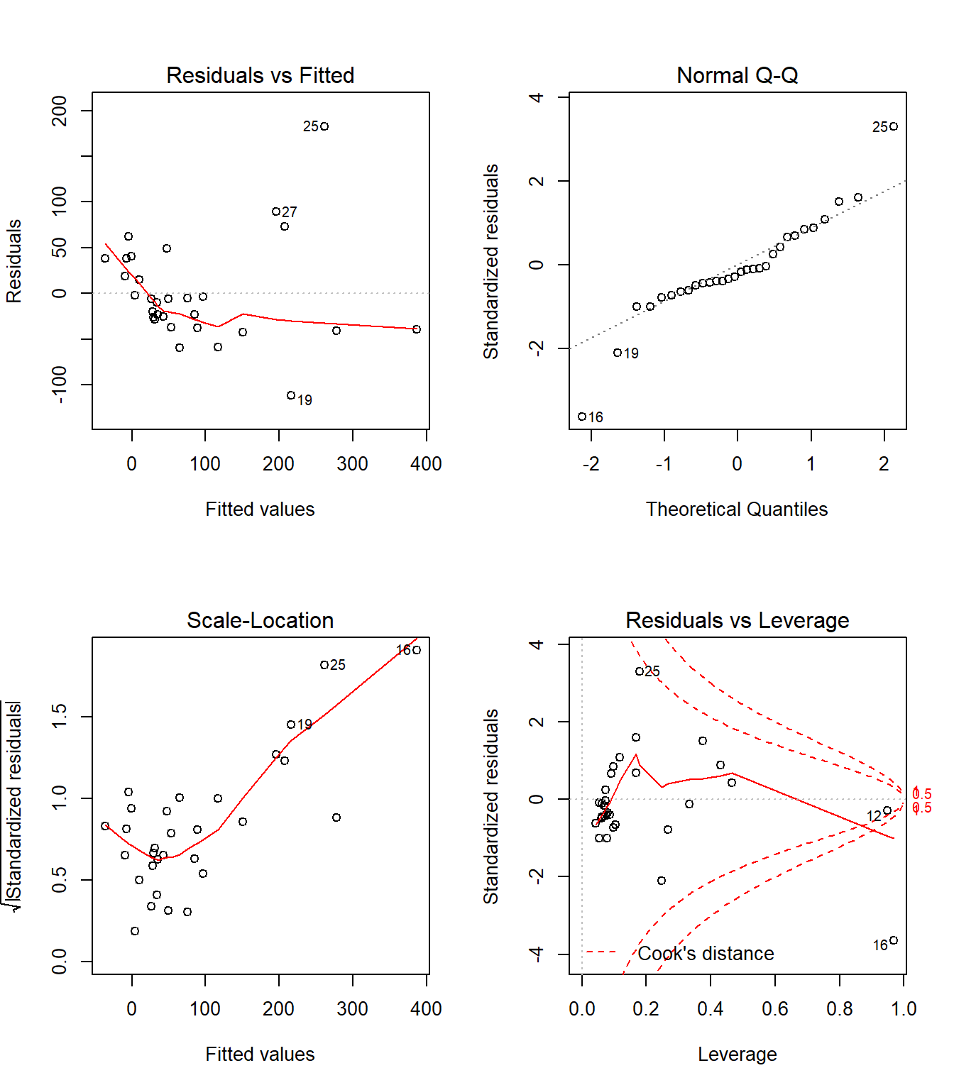
46.12 Model 1: Diagnostic Plot 1

As we’ve seen, the first of R’s automated diagnostic plots for a linear model is a plot of the residuals vs. the fitted values.

plot(model1, which=1)

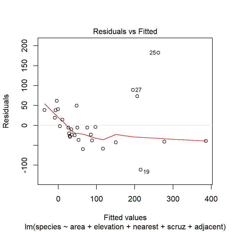
46.12.1 Questions about Diagnostic Plot 1: Residuals vs. Fitted Values

What type of regression residuals is R plotting here?
Which points are identified by numbers here?
Why did R include the gray dotted line at Residual = 0?
What is the purpose of the thin red line?
What can you tell about the potential for outliers in the model 1 residuals from the plot?
What are we looking for in this plot that would let us conclude there were no important assumption violations implied by it? Which assumptions can we assess with it?
What would we do if we saw a violation of assumptions in this plot?
What are the key differences between this plot and the one I showed earlier?

46.13 Diagnostic Plot 2: Assessing Normality

The second diagnostic plot prepared by R for any linear model using the plot command is a Normal Q-Q plot of the standardized residuals from the model.

plot(model1, which=2)

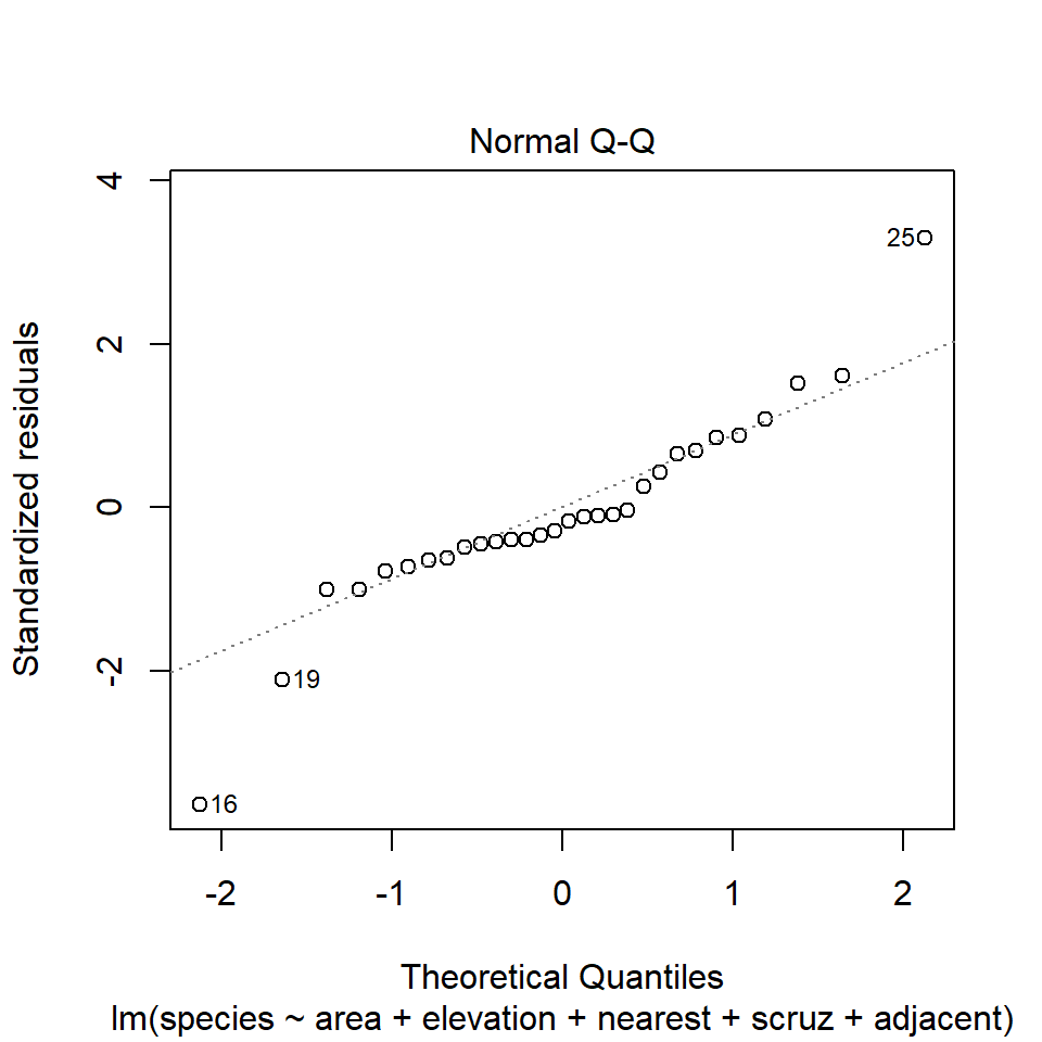
46.13.1 Questions about Diagnostic Plot 2: Normal Plot of Standardized Residuals

Which points are being identified here by number?
Which assumption(s) of multiple regression does this plot help us check?
What are we looking for in this plot that would let us conclude there were no important assumption violations implied by it?
What would we do if we saw a violation of assumptions in this plot?

We could also look at studentized residuals, or we could apply a more complete set of plots and other assessments of normality. Usually, I don’t.

46.14 Diagnostic Plot 3: Assessing Constant Variance

The third diagnostic plot prepared by R for any linear model using the plot command shows the square root of the model’s standardized residuals vs. its fitted values. R calls this a scale-location plot.

plot(model1, which=3)

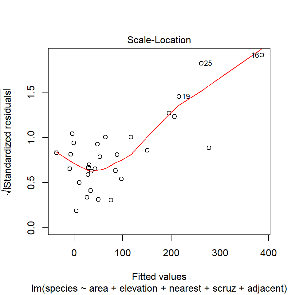
46.14.1 Questions about Diagnostic Plot 3: Scale-Location Plot

Which points are being identified here by number?
Which assumption(s) of multiple regression does this plot help us check?
What is the role of the thin red line in this plot?
What are we looking for in this plot that would let us conclude there were no important assumption violations implied by it?
What would we do if we saw a violation of assumptions in this plot?

46.15 Obtaining Fitted Values and Residuals from a Model

Remember that we can use the fitted function applied to a model to find the predictions made by the regression model for each of the observations used to create the model.

round(fitted(model1),2)

     1      2      3      4      5      6      7      8      9     10 
116.73  -7.27  29.33  10.36 -36.38  43.09  33.92  -9.02  28.31  30.79 
    11     12     13     14     15     16     17     18     19     20 
 47.66  96.99  -4.03  64.63  -0.50 386.40  88.69   4.04 215.68 150.48 
    21     22     23     24     25     26     27     28     29     30 
 35.08  75.55 206.95 277.68 261.42  85.38 195.62  49.81  52.94  26.70

gala[1,]

# A tibble: 1 x 10
     id island species  area elevation nearest scruz adjacent stures  fits
  <int> <fct>    <int> <dbl>     <int>   <dbl> <dbl>    <dbl>  <dbl> <dbl>
1     1 Baltra      58  25.1       346     0.6   0.6     1.84  -1.00  117.

46.15.1 Questions about Fitted Values

Verify that the first fitted value [116.73] is in fact what you get for Baltra (observation 1) when you apply the regression equation:

species = 7.07 - 0.02 area + 0.32 elevation 
               + 0.009 nearest - 0.24 scruz - 0.07 adjacent

We can compare these predictions to the actual observed counts of the number of species on each island. Subtracting the fitted values from the observed values gives us the residuals, as does the resid function.

round(resid(model1),2)

      1       2       3       4       5       6       7       8       9 
 -58.73   38.27  -26.33   14.64   38.38  -25.09   -9.92   19.02  -20.31 
     10      11      12      13      14      15      16      17      18 
 -28.79   49.34   -3.99   62.03  -59.63   40.50  -39.40  -37.69   -2.04 
     19      20      21      22      23      24      25      26      27 
-111.68  -42.48  -23.08   -5.55   73.05  -40.68  182.58  -23.38   89.38 
     28      29      30 
  -5.81  -36.94   -5.70

46.15.2 Questions about Residuals

What does a positive residual indicate?
What does a negative residual indicate?
The standard deviation of the full set of 30 residuals turns out to be 55.47. How does this compare to the residual standard error?
The command below identifies Santa Cruz. What does it indicate about Santa Cruz, specifically?

gala$island[which.max(resid(model1))]

[1] SantaCruz
30 Levels: Baltra Bartolome Caldwell Champion Coamano ... Wolf

From the results below, what is the model1 residual for Santa Cruz? What does this imply about the species prediction made by Model 1 for Santa Cruz?

which.max(resid(model1))

25 
25

round(resid(model1),2)

      1       2       3       4       5       6       7       8       9 
 -58.73   38.27  -26.33   14.64   38.38  -25.09   -9.92   19.02  -20.31 
     10      11      12      13      14      15      16      17      18 
 -28.79   49.34   -3.99   62.03  -59.63   40.50  -39.40  -37.69   -2.04 
     19      20      21      22      23      24      25      26      27 
-111.68  -42.48  -23.08   -5.55   73.05  -40.68  182.58  -23.38   89.38 
     28      29      30 
  -5.81  -36.94   -5.70

gala[which.max(resid(model1)),]

# A tibble: 1 x 10
     id island species  area elevation nearest scruz adjacent stures  fits
  <int> <fct>    <int> <dbl>     <int>   <dbl> <dbl>    <dbl>  <dbl> <dbl>
1    25 Santa~     444  904.       864     0.6     0     0.52   4.38  261.

46.16 Relationship between Fitted and Observed Values

We’ve already seen that the fitted command can produce predicted values for each observations used to develop a regression model, and that the resid command can produce the residuals (observed - predicted) for those same observations. Returning to our original model1, let’s compare the fitted values (stored earlier in fits) to the observed values.

ggplot(gala, aes(x = species, y = fits)) +
    geom_point(size = 3, shape = 1) + theme_bw() +
    geom_abline(intercept = 0, slope = 1, col = "purple", linetype = "dashed") +
    labs(x = "Observed Species Count", y = "Model Predicted Species")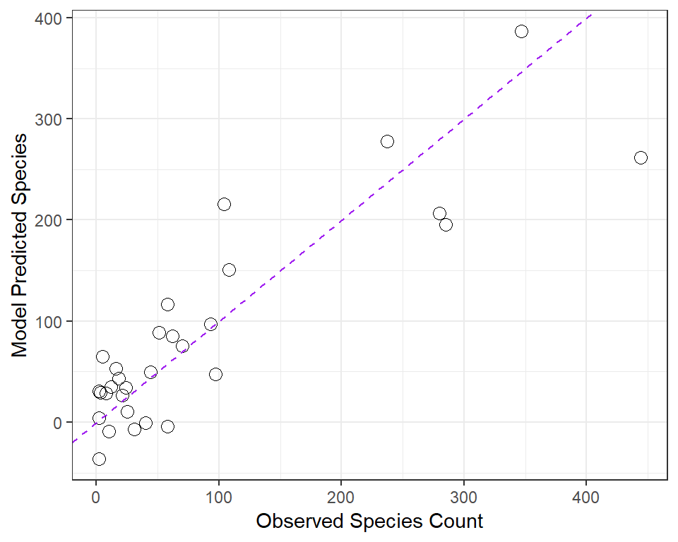

46.16.1 Questions about Fitted and Observed Values

Why did I draw the dotted purple line with y-intercept 0 and slope 1? Why is that particular line of interest?
If a point on this plot is in the top left here, above the dotted line, what does that mean?
If a point is below the dotted line here, what does that mean?
How does this plot display the size of an observation’s residual?

46.17 Standardizing Residuals

We’ve already seen that the raw residuals from a regression model can be obtained using the resid function. Residuals are defined to have mean 0. This is one of the requirements of the least squares procedure for estimating a linear model, and their true standard deviation is effectively estimated using the residual standard error.

There are two additional types of residuals for us to be aware of: standardized residuals, and studentized (sometimes called externally standardized, or jackknife) residuals. Each approach standardizes the residuals by dividing them by a standard deviation estimate, so the resulting residuals should have mean 0 and standard deviation 1 if assumptions hold.

Standardized residuals are the original (raw) residuals, scaled by a standard deviation estimate developed using the entire data set.
Studentized residuals are the original (raw) residuals, scaled by a standard deviation estimate developed using the entire data set EXCEPT for this particular observation.

The rstandard function, when applied to a linear regression model, will generate the standardized residuals, while rstudent generates the model’s studentized residuals.

`geom_smooth()` using method = 'loess' and formula 'y ~ x'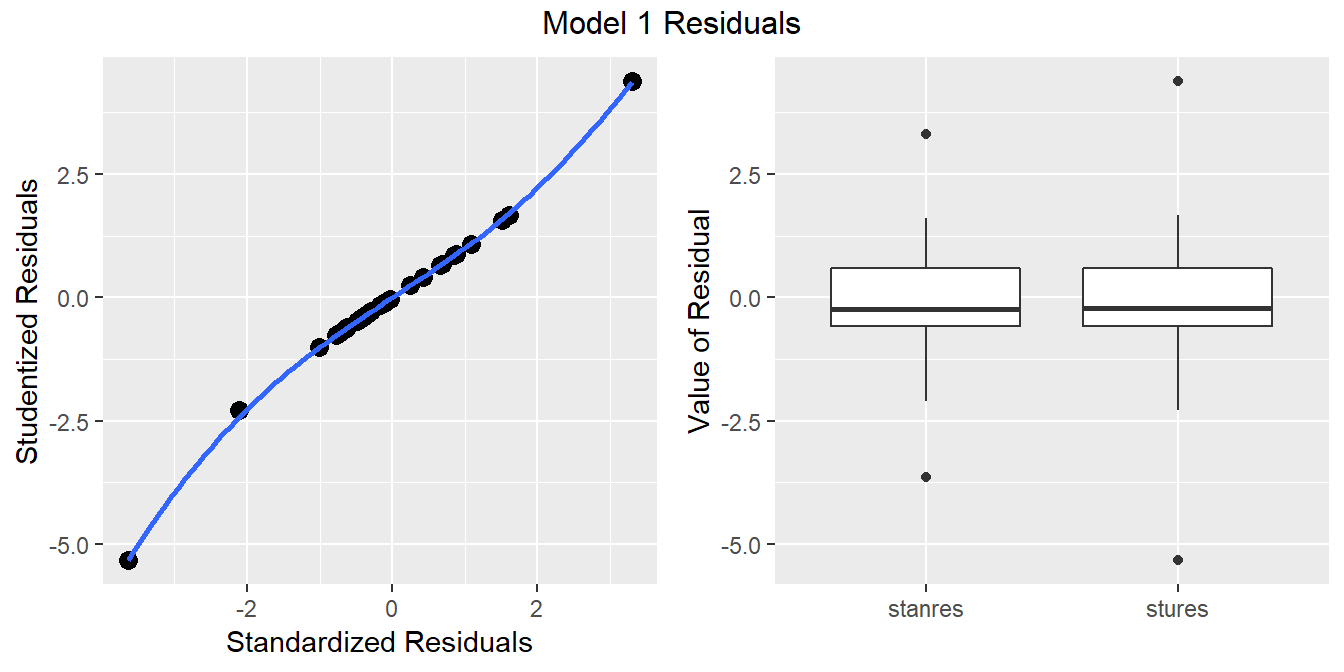

46.17.1 Questions about Standardized and Studentized Residuals

From the plots above, what conclusions can you draw about the two methods of standardizing residuals as they apply in the case of our model1?

46.18 Three Types of Residuals

gala.res <- data.frame(raw.residuals = resid(model1),
                       standardized = rstandard(model1),
                       studentized = rstudent(model1)) %>% tbl_df

gala.res_long <- gather(gala.res, key = "type", value = "res")
ggplot(gala.res_long, aes(x = type, y = res)) + 
    geom_boxplot() + 
    coord_flip() + 
    labs(x = "", y = "Residual", title = "3 Types of Residuals for Model 1")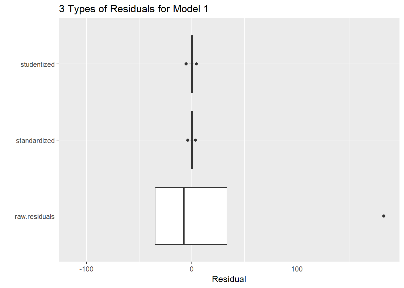

46.18.1 Questions about Three Types of Residuals

Consider the three types of residuals, shown above. Can you specify a reason why looking at the raw residuals might be helpful in this case?
Why might (either of the two approaches to) standardizing be useful?
Does there seem to be a substantial problem with Normality in the residuals?
How about the Normality of the studentized residuals? Which seems clearer?

References

Faraway, Julian J. 2015. Linear Models with R. Second. Boca Raton, FL: CRC Press.