Chapter 13 The Western Collaborative Group Study
13.1 The Western Collaborative Group Study (wcgs) data set
Vittinghoff et al. (2012) explore data from the Western Collaborative Group Study (WCGS) in great detail9. We’ll touch lightly on some key issues in this Chapter.
# A tibble: 3,154 x 22
      id   age agec  height weight lnwght wghtcat   bmi   sbp lnsbp   dbp
   <int> <int> <fct>  <int>  <int>  <dbl> <fct>   <dbl> <int> <dbl> <int>
 1  2343    50 46-50     67    200   5.30 170-200  31.3   132  4.88    90
 2  3656    51 51-55     73    192   5.26 170-200  25.3   120  4.79    74
 3  3526    59 56-60     70    200   5.30 170-200  28.7   158  5.06    94
 4 22057    51 51-55     69    150   5.01 140-170  22.1   126  4.84    80
 5 12927    44 41-45     71    160   5.08 140-170  22.3   126  4.84    80
 6 16029    47 46-50     64    158   5.06 140-170  27.1   116  4.75    76
 7  3894    40 35-40     70    162   5.09 140-170  23.2   122  4.80    78
 8 11389    41 41-45     70    160   5.08 140-170  23.0   130  4.87    84
 9 12681    50 46-50     71    195   5.27 170-200  27.2   112  4.72    70
10 10005    43 41-45     68    187   5.23 170-200  28.4   120  4.79    80
# ... with 3,144 more rows, and 11 more variables: chol <int>,
#   behpat <fct>, dibpat <fct>, smoke <fct>, ncigs <int>, arcus <int>,
#   chd69 <fct>, typchd69 <int>, time169 <int>, t1 <dbl>, uni <dbl>
Here, we have 3154 rows (subjects) and 22 columns (variables).
13.1.1 Structure of wcgs
We can specify the (sometimes terrible) variable names, through the names function, or we can add other elements of the structure, so that we can identify elements of particular interest.
Classes 'tbl_df', 'tbl' and 'data.frame':   3154 obs. of  22 variables:
 $ id      : int  2343 3656 3526 22057 12927 16029 3894 11389 12681 10005 ...
 $ age     : int  50 51 59 51 44 47 40 41 50 43 ...
 $ agec    : Factor w/ 5 levels "35-40","41-45",..: 3 4 5 4 2 3 1 2 3 2 ...
 $ height  : int  67 73 70 69 71 64 70 70 71 68 ...
 $ weight  : int  200 192 200 150 160 158 162 160 195 187 ...
 $ lnwght  : num  5.3 5.26 5.3 5.01 5.08 ...
 $ wghtcat : Factor w/ 4 levels "< 140","> 200",..: 4 4 4 3 3 3 3 3 4 4 ...
 $ bmi     : num  31.3 25.3 28.7 22.1 22.3 ...
 $ sbp     : int  132 120 158 126 126 116 122 130 112 120 ...
 $ lnsbp   : num  4.88 4.79 5.06 4.84 4.84 ...
 $ dbp     : int  90 74 94 80 80 76 78 84 70 80 ...
 $ chol    : int  249 194 258 173 214 206 190 212 130 233 ...
 $ behpat  : Factor w/ 4 levels "A1","A2","B3",..: 1 1 1 1 1 1 1 1 1 1 ...
 $ dibpat  : Factor w/ 2 levels "Type A","Type B": 1 1 1 1 1 1 1 1 1 1 ...
 $ smoke   : Factor w/ 2 levels "No","Yes": 2 2 1 1 1 2 1 2 1 2 ...
 $ ncigs   : int  25 25 0 0 0 80 0 25 0 25 ...
 $ arcus   : int  1 0 1 1 0 0 0 0 1 0 ...
 $ chd69   : Factor w/ 2 levels "No","Yes": 1 1 1 1 1 1 1 1 1 1 ...
 $ typchd69: int  0 0 0 0 0 0 0 0 0 0 ...
 $ time169 : int  1367 2991 2960 3069 3081 2114 2929 3010 3104 2861 ...
 $ t1      : num  -1.63 -4.06 0.64 1.12 2.43 ...
 $ uni     : num  0.486 0.186 0.728 0.624 0.379 ...
13.1.2 Codebook for wcgs
This table was lovingly hand-crafted, and involved a lot of typing. We’ll look for better ways in 432.
| Name | Stored As | Type | Details (units, levels, etc.) |
|---|---|---|---|
id |
integer | (nominal) | ID #, nominal and uninteresting |
age |
integer | quantitative | age, in years - no decimal places |
agec |
factor (5) | (ordinal) | age: 35-40, 41-45, 46-50, 51-55, 56-60 |
height |
integer | quantitative | height, in inches |
weight |
integer | quantitative | weight, in pounds |
lnwght |
number | quantitative | natural logarithm of weight |
wghtcat |
factor (4) | (ordinal) | wt: < 140, 140-170, 170-200, > 200 |
bmi |
number | quantitative | body-mass index: |
| 703 * weight in lb / (height in in)2 | |||
sbp |
integer | quantitative | systolic blood pressure, in mm Hg |
lnsbp |
number | quantitative | natural logarithm of sbp |
dbp |
integer | quantitative | diastolic blood pressure, mm Hg |
chol |
integer | quantitative | total cholesterol, mg/dL |
behpat |
factor (4) | (nominal) | behavioral pattern: A1, A2, B3 or B4 |
dibpat |
factor (2) | (binary) | behavioral pattern: A or B |
smoke |
factor (2) | (binary) | cigarette smoker: Yes or No |
ncigs |
integer | quantitative | number of cigarettes smoked per day |
arcus |
integer | (nominal) | arcus senilis present (1) or absent (0) |
chd69 |
factor (2) | (binary) | CHD event: Yes or No |
typchd69 |
integer | (4 levels) | event: 0 = no CHD, 1 = MI or SD, |
| 2 = silent MI, 3 = angina | |||
time169 |
integer | quantitative | follow-up time in days |
t1 |
number | quantitative | heavy-tailed (random draws) |
uni |
number | quantitative | light-tailed (random draws) |
13.1.3 Quick Summary
       id             age          agec          height         weight
 Min.   : 2001   Min.   :39.0   35-40: 543   Min.   :60.0   Min.   : 78
 1st Qu.: 3741   1st Qu.:42.0   41-45:1091   1st Qu.:68.0   1st Qu.:155
 Median :11406   Median :45.0   46-50: 750   Median :70.0   Median :170
 Mean   :10478   Mean   :46.3   51-55: 528   Mean   :69.8   Mean   :170
 3rd Qu.:13115   3rd Qu.:50.0   56-60: 242   3rd Qu.:72.0   3rd Qu.:182
 Max.   :22101   Max.   :59.0                Max.   :78.0   Max.   :320

     lnwght        wghtcat          bmi            sbp          lnsbp
 Min.   :4.36   < 140  : 232   Min.   :11.2   Min.   : 98   Min.   :4.58
 1st Qu.:5.04   > 200  : 213   1st Qu.:23.0   1st Qu.:120   1st Qu.:4.79
 Median :5.14   140-170:1538   Median :24.4   Median :126   Median :4.84
 Mean   :5.13   170-200:1171   Mean   :24.5   Mean   :129   Mean   :4.85
 3rd Qu.:5.20                  3rd Qu.:25.8   3rd Qu.:136   3rd Qu.:4.91
 Max.   :5.77                  Max.   :38.9   Max.   :230   Max.   :5.44

      dbp           chol     behpat       dibpat     smoke
 Min.   : 58   Min.   :103   A1: 264   Type A:1589   No :1652
 1st Qu.: 76   1st Qu.:197   A2:1325   Type B:1565   Yes:1502
 Median : 80   Median :223   B3:1216
 Mean   : 82   Mean   :226   B4: 349
 3rd Qu.: 86   3rd Qu.:253
 Max.   :150   Max.   :645
               NA's   :12
     ncigs          arcus       chd69         typchd69        time169
 Min.   : 0.0   Min.   :0.000   No :2897   Min.   :0.000   Min.   :  18
 1st Qu.: 0.0   1st Qu.:0.000   Yes: 257   1st Qu.:0.000   1st Qu.:2842
 Median : 0.0   Median :0.000              Median :0.000   Median :2942
 Mean   :11.6   Mean   :0.299              Mean   :0.136   Mean   :2684
 3rd Qu.:20.0   3rd Qu.:1.000              3rd Qu.:0.000   3rd Qu.:3037
 Max.   :99.0   Max.   :1.000              Max.   :3.000   Max.   :3430
                NA's   :2
       t1             uni
 Min.   :-47.4   Min.   :0.001
 1st Qu.: -1.0   1st Qu.:0.257
 Median :  0.0   Median :0.516
 Mean   :  0.0   Mean   :0.505
 3rd Qu.:  1.0   3rd Qu.:0.756
 Max.   : 47.0   Max.   :0.999
 NA's   :39
For a more detailed description, we might consider Hmisc::describe, psych::describe, mosaic::favstats, etc.
13.2 Are the SBPs Normally Distributed?
Consider the question of whether the distribution of the systolic blood pressure results is well-approximated by the Normal.
ggplot(wcgs, aes(x = sbp)) +
    geom_histogram(aes(y = ..density..),
                   bins = 30, fill = "aquamarine", col="blue") +
    stat_function(fun = dnorm, lwd = 1.5, col = "darkblue",
                  args = list(mean = mean(wcgs$sbp), sd = sd(wcgs$sbp))) +
    annotate("text", x = 200, y = 0.01, col = "darkblue",
             label = paste("Mean = ", round(mean(wcgs$sbp),1),
                           ", SD = ", round(sd(wcgs$sbp),1))) +
    labs(title = "Systolic BP for `wcgs` subjects",
         caption = "Histogram with Normal Density superimposed")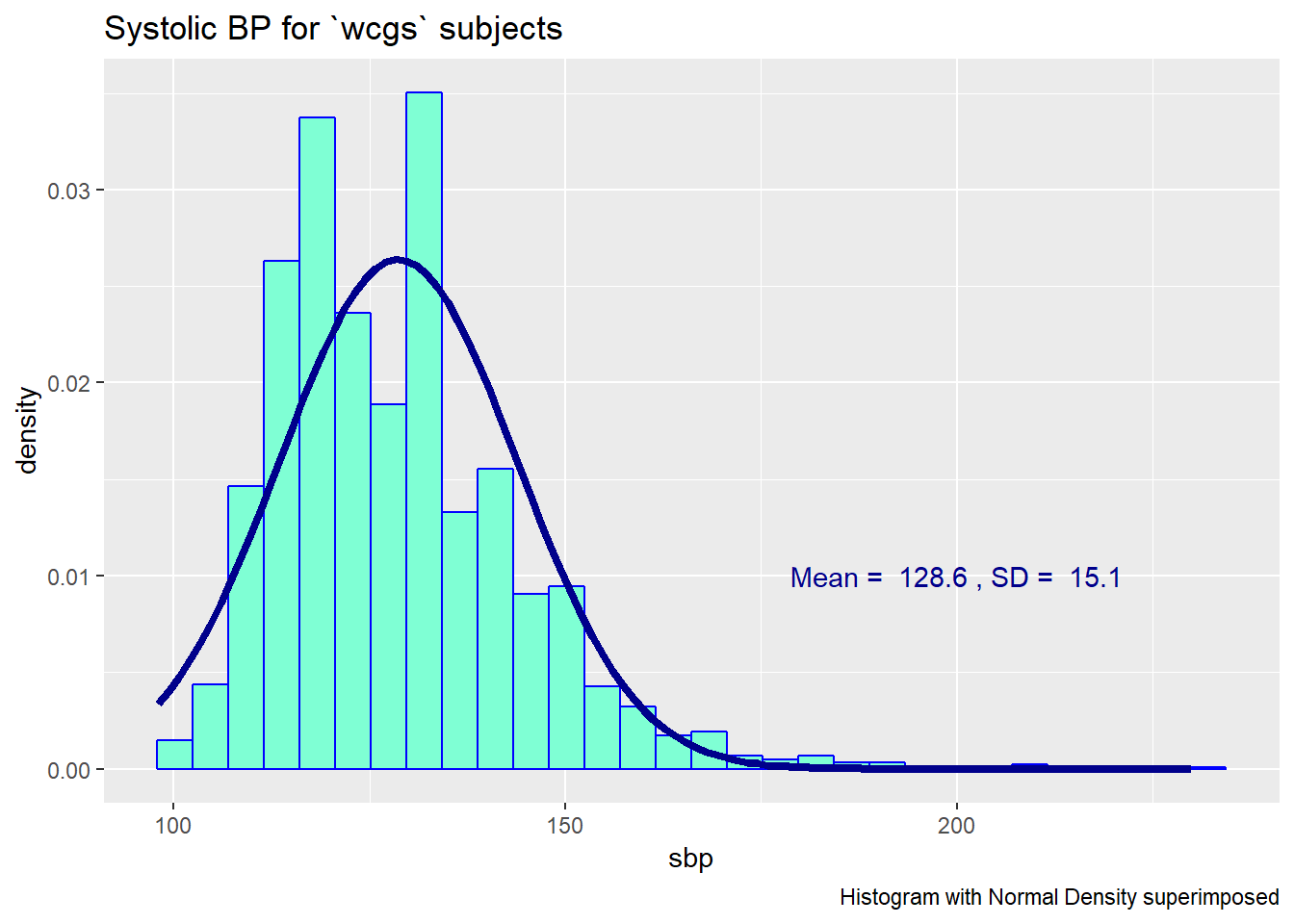
Since the data contain both sbp and lnsbp (its natural logarithm), let’s compare them. Note that in preparing the graph, we’ll need to change the location for the text annotation.
ggplot(wcgs, aes(x = lnsbp)) +
    geom_histogram(aes(y = ..density..),
                   bins = 30, fill = "aquamarine", col="blue") +
    stat_function(fun = dnorm, lwd = 1.5, col = "darkblue",
                  args = list(mean = mean(wcgs$lnsbp),
                              sd = sd(wcgs$lnsbp))) +
    annotate("text", x = 5.2, y = 2, col = "darkblue",
             label = paste("Mean = ", round(mean(wcgs$lnsbp),1),
                           ", SD = ", round(sd(wcgs$lnsbp),1))) +
    labs(title = "Natural Logarithm of `wcgs` Systolic BP",
         caption = "Histogram with Normal Density superimposed")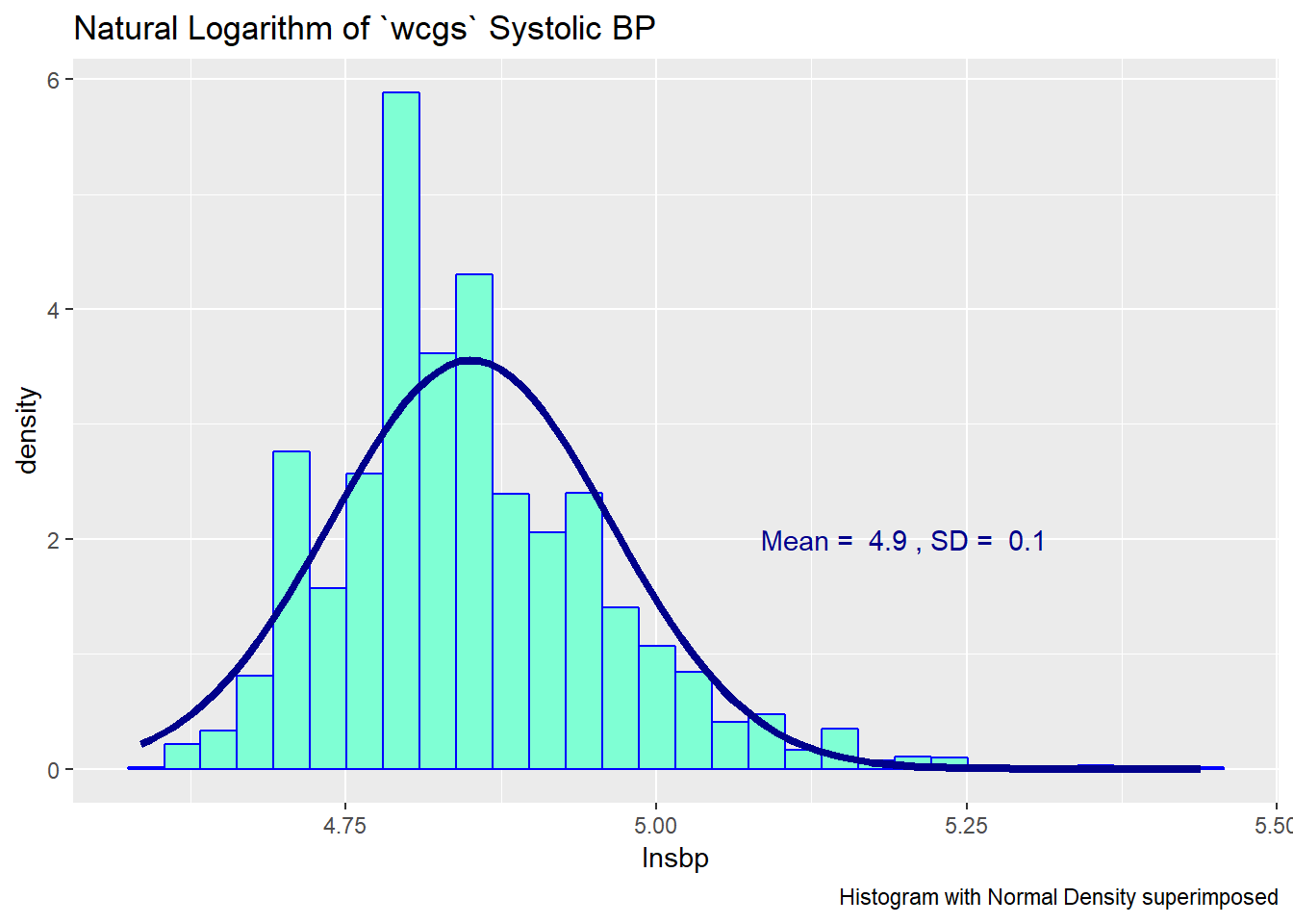
We can also look at Normal Q-Q plots, for instance…
p1 <- ggplot(wcgs, aes(sample = sbp)) +
    geom_point(stat="qq", color = "orchid") +
    labs(y = "Ordered SBP", title = "sbp in wcgs")

p2 <- ggplot(wcgs, aes(sample = lnsbp)) +
    geom_point(stat="qq", color = "orange") +
    labs(y = "Ordered ln(sbp)", title = "ln(sbp) in wcgs")

gridExtra::grid.arrange(p1, p2, ncol=2, top ="Normal Q-Q plots of SBP and ln(SBP) in wcgs")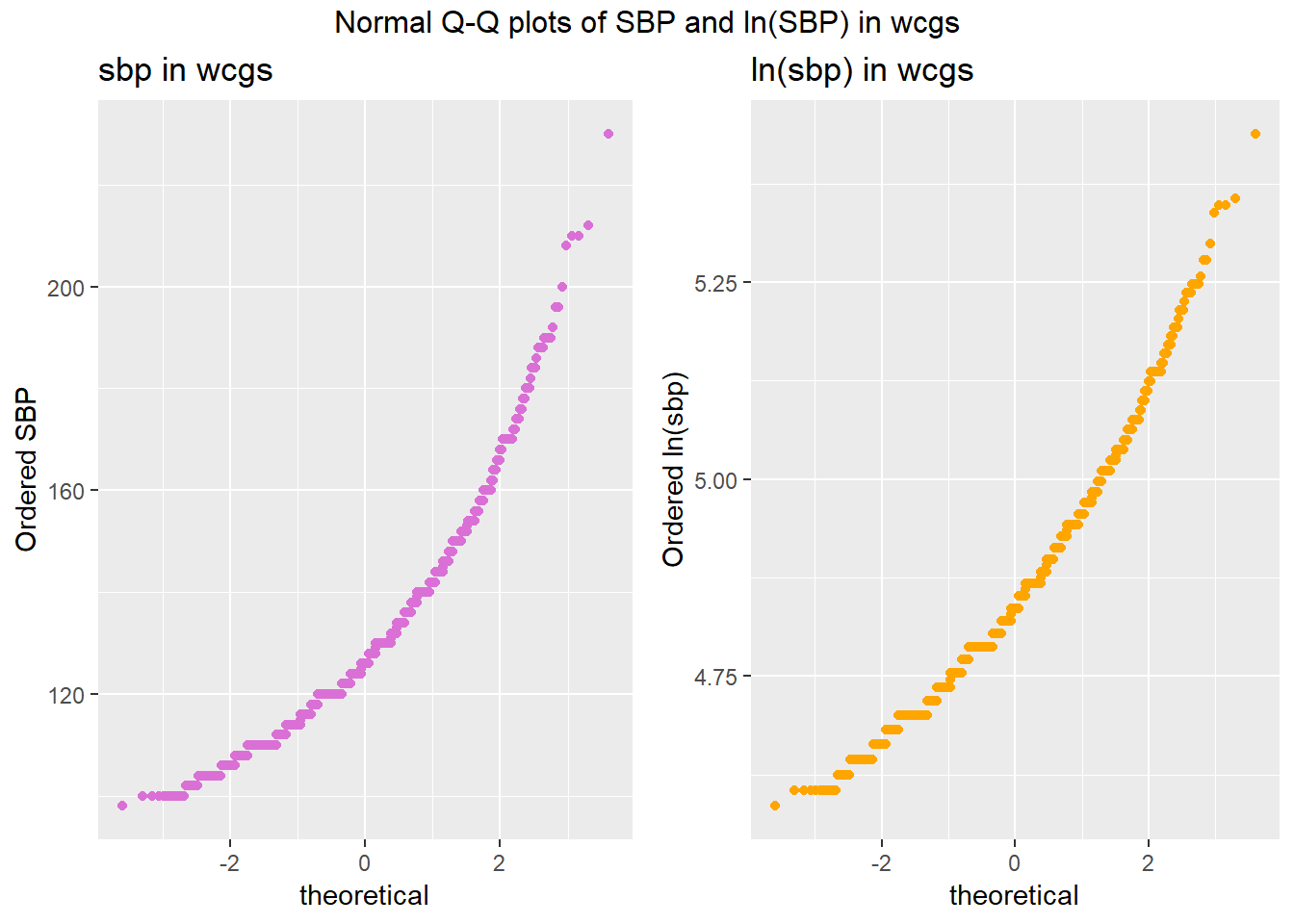
There’s at best a small improvement from sbp to lnsbp in terms of approximation by a Normal distribution.
13.3 Describing Outlying Values with Z Scores
It looks like there’s an outlier (or a series of them) in the SBP data.
ggplot(wcgs, aes(x = 1, y = sbp)) +
    geom_boxplot(fill = "royalblue") +
    labs(title = "Boxplot of SBP in `wcgs` data",
         y = "Systolic Blood Pressure (mm Hg)",
         x = "") +
    theme(axis.text.y = element_blank(),
          axis.ticks.y = element_blank()) +
coord_flip() 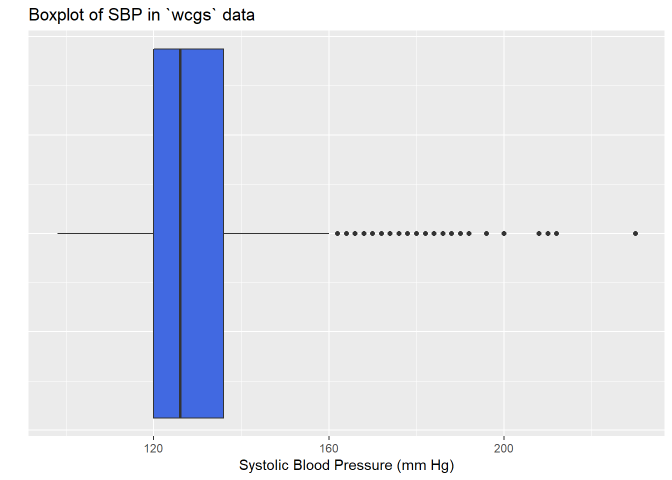
wcgs$sbp
       n  missing distinct     Info     Mean      Gmd      .05      .10
    3154        0       62    0.996    128.6    16.25      110      112
     .25      .50      .75      .90      .95
     120      126      136      148      156

lowest :  98 100 102 104 106, highest: 200 208 210 212 230
The maximum value here is 230, and is clearly the most extreme value in the data set. One way to gauge this is to describe that observation’s Z score, the number of standard deviations away from the mean that the observation falls. Here, the maximum value, 230 is 6.71 standard deviations above the mean, and thus has a Z score of 6.7.
A negative Z score would indicate a point below the mean, while a positive Z score indicates, as we’ve seen, a point above the mean. The minimum systolic blood pressure, 98 is 2.03 standard deviations below the mean, so it has a Z score of -2.
Recall that the Empirical Rule suggests that if a variable follows a Normal distribution, it would have approximately 95% of its observations falling inside a Z score of (-2, 2), and 99.74% falling inside a Z score range of (-3, 3). Do the systolic blood pressures appear Normally distributed?
13.4 Does Weight Category Relate to SBP?
The data are collected into four groups based on the subject’s weight (in pounds).
ggplot(wcgs, aes(x = wghtcat, y = sbp, fill = wghtcat)) +
    geom_boxplot(notch = TRUE) +
    scale_fill_viridis(discrete=TRUE) +
    guides(fill = FALSE) +
    labs(title = "Boxplot of Systolic BP by Weight Category in WCGS",
         x = "Weight Category", y = "Systolic Blood Pressure")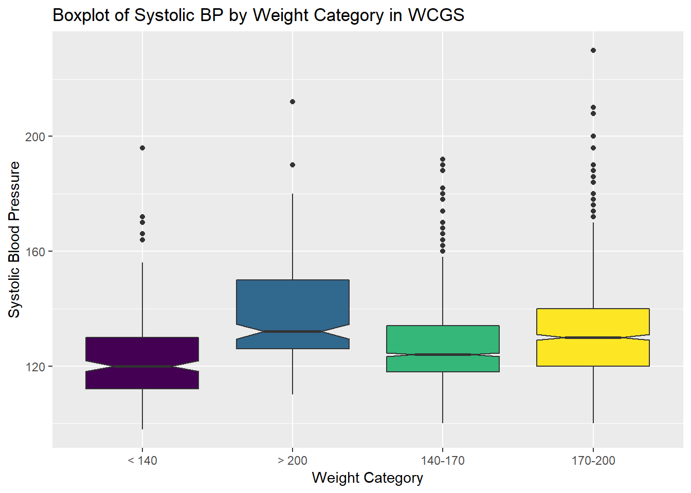
13.5 Re-Leveling a Factor
Well, that’s not so good. We really want those weight categories (the levels) to be ordered more sensibly.
  < 140   > 200 140-170 170-200
    232     213    1538    1171
Like all factor variables in R, the categories are specified as levels.
[1] "< 140" "> 200" "140-170" "170-200"We want to change the order of the levels in a new version of this factor variable so they make sense. There are multiple ways to do this, but I prefer the fct_relevel function from the forcats package. Which order is more appropriate?
          < 140 > 200 140-170 170-200
  < 140     232     0       0       0
  140-170     0     0    1538       0
  170-200     0     0       0    1171
  > 200       0   213       0       0
I’ll add a new variable to the wcgs data called weight_f that relevels the wghtcat data.
wcgs <- wcgs %>%
    mutate(weight_f = fct_relevel(wghtcat, "< 140", "140-170", "170-200", "> 200"))

table(wcgs$weight_f)
  < 140 140-170 170-200   > 200
    232    1538    1171     213
For more on the forcats package, check out Grolemund and Wickham (2017), especially the Section on Factors.
13.5.1 SBP by Weight Category
ggplot(wcgs, aes(x = weight_f, y = sbp, fill = weight_f)) +
    geom_boxplot(notch = TRUE) +
    scale_fill_viridis(discrete=TRUE) +
    guides(fill = FALSE) +
    labs(title = "Systolic Blood Pressure by Reordered Weight Category in WCGS",
         x = "Weight Category", y = "Systolic Blood Pressure")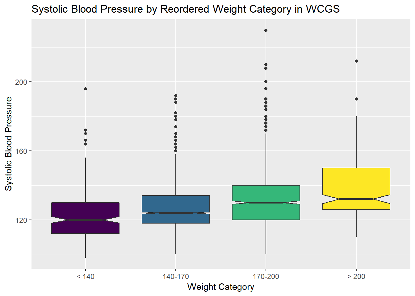
We might see some details well with a ridgeline plot, too.
wcgs %>%
    ggplot(aes(x = sbp, y = weight_f, fill = weight_f, height = ..density..)) +
    ggridges::geom_density_ridges(scale = 2) +
    scale_fill_viridis(discrete = TRUE) +
    guides(fill = FALSE) +
    labs(title = "SBP by Weight Category (wcgs)",
         x = "Systolic Blood Pressure",
         y = "Weight Category") +
    theme_bw()
Picking joint bandwidth of 3.74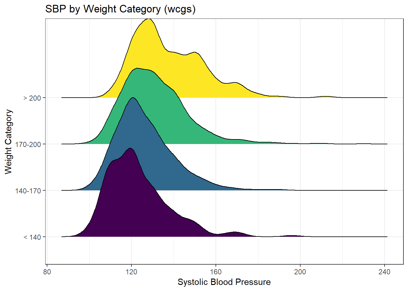
As the plots suggest, patients in the heavier groups generally had higher systolic blood pressures.
wcgs$weight_f: < 140
 min  Q1 median  Q3 max mean   sd   n missing
  98 112    120 130 196  123 14.7 232       0
--------------------------------------------------------
wcgs$weight_f: 140-170
 min  Q1 median  Q3 max mean   sd    n missing
 100 118    124 134 192  126 13.7 1538       0
--------------------------------------------------------
wcgs$weight_f: 170-200
 min  Q1 median  Q3 max mean   sd    n missing
 100 120    130 140 230  131 15.6 1171       0
--------------------------------------------------------
wcgs$weight_f: > 200
 min  Q1 median  Q3 max mean   sd   n missing
 110 126    132 150 212  138 16.8 213       0
13.6 Are Weight and SBP Linked?
Let’s build a scatter plot of SBP (Outcome) by Weight (Predictor), rather than breaking down into categories.
ggplot(wcgs, aes(x = weight, y = sbp)) +
    geom_point(size=3, shape=1, color="forestgreen") + ## default size = 2
    stat_smooth(method=lm, color="red") + ## add se=FALSE to hide conf. interval
    stat_smooth(method=loess, se=FALSE, color="blue") +
    ggtitle("SBP vs. Weight in 3,154 WCGS Subjects") +
    theme_bw()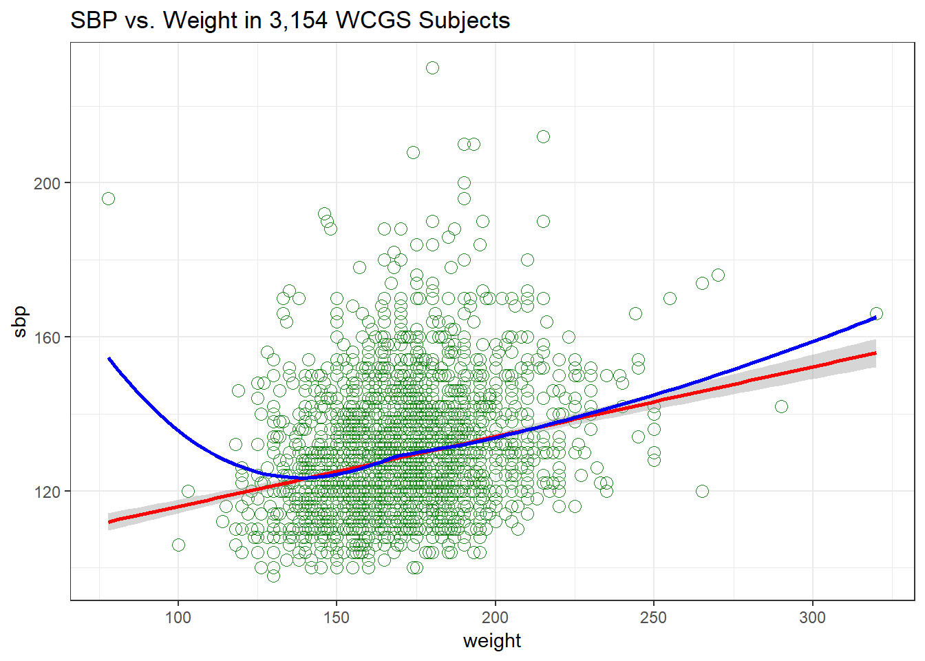
- The mass of the data is hidden from us - showing 3154 points in one plot can produce little more than a blur where there are lots of points on top of each other.
- Here the least squares regression line (in red), and loess scatterplot smoother, (in blue) can help.
The relationship between systolic blood pressure and weight appears to be very close to linear, but of course there is considerable scatter around that generally linear relationship. It turns out that the Pearson correlation of these two variables is 0.253.
13.7 SBP and Weight by Arcus Senilis groups?
An issue of interest to us will be to assess whether the SBP-Weight relationship we see above is similar among subjects who have arcus senilis and those who do not.
Arcus senilis is an old age syndrome where there is a white, grey, or blue opaque ring in the corneal margin (peripheral corneal opacity), or white ring in front of the periphery of the iris. It is present at birth but then fades; however, it is quite commonly present in the elderly. It can also appear earlier in life as a result of hypercholesterolemia.
Wikipedia article on Arcus Senilis, retrieved 2017-08-15
Let’s start with a quick look at the arcus data.
     arcus
 Min.   :0.000
 1st Qu.:0.000
 Median :0.000
 Mean   :0.299
 3rd Qu.:1.000
 Max.   :1.000
 NA's   :2
We have 2 missing values, so we probably want to do something about that before plotting the data, and we may also want to create a factor variable with more meaningful labels than 1 (which means yes, arcus senilis is present) and 0 (which means no, it isn’t.) We’ll use the
wcgs <- wcgs %>%
    mutate(arcus_f = fct_recode(factor(arcus),
                                "Arcus senilis" = "1",
                                "No arcus senilis" = "0"),
           arcus_f = fct_relevel(arcus_f, "Arcus senilis"))

table(wcgs$arcus_f, wcgs$arcus, useNA = "ifany")
                      0    1 <NA>
  Arcus senilis       0  941    0
  No arcus senilis 2211    0    0
  <NA>                0    0    2
Let’s build a version of the wcgs data that eliminates all missing data in the variables of immediate interest, and then plot the SBP-weight relationship in groups of patients with and without arcus senilis.
wcgs %>%
    filter(complete.cases(arcus_f, sbp, weight)) %>%
    ggplot(aes(x = weight, y = sbp, group = arcus_f)) +
    geom_point(size=3, shape = 1) +
    stat_smooth(method=lm, color="red") +
    stat_smooth(method=loess, se=FALSE, color="blue") +
    labs(title = "SBP vs. Weight by Arcus Senilis status",
         caption = "3,152 Western Collaborative Group Study subjects with known arcus senilis status") +
    facet_wrap(~ arcus_f) +
    theme_bw()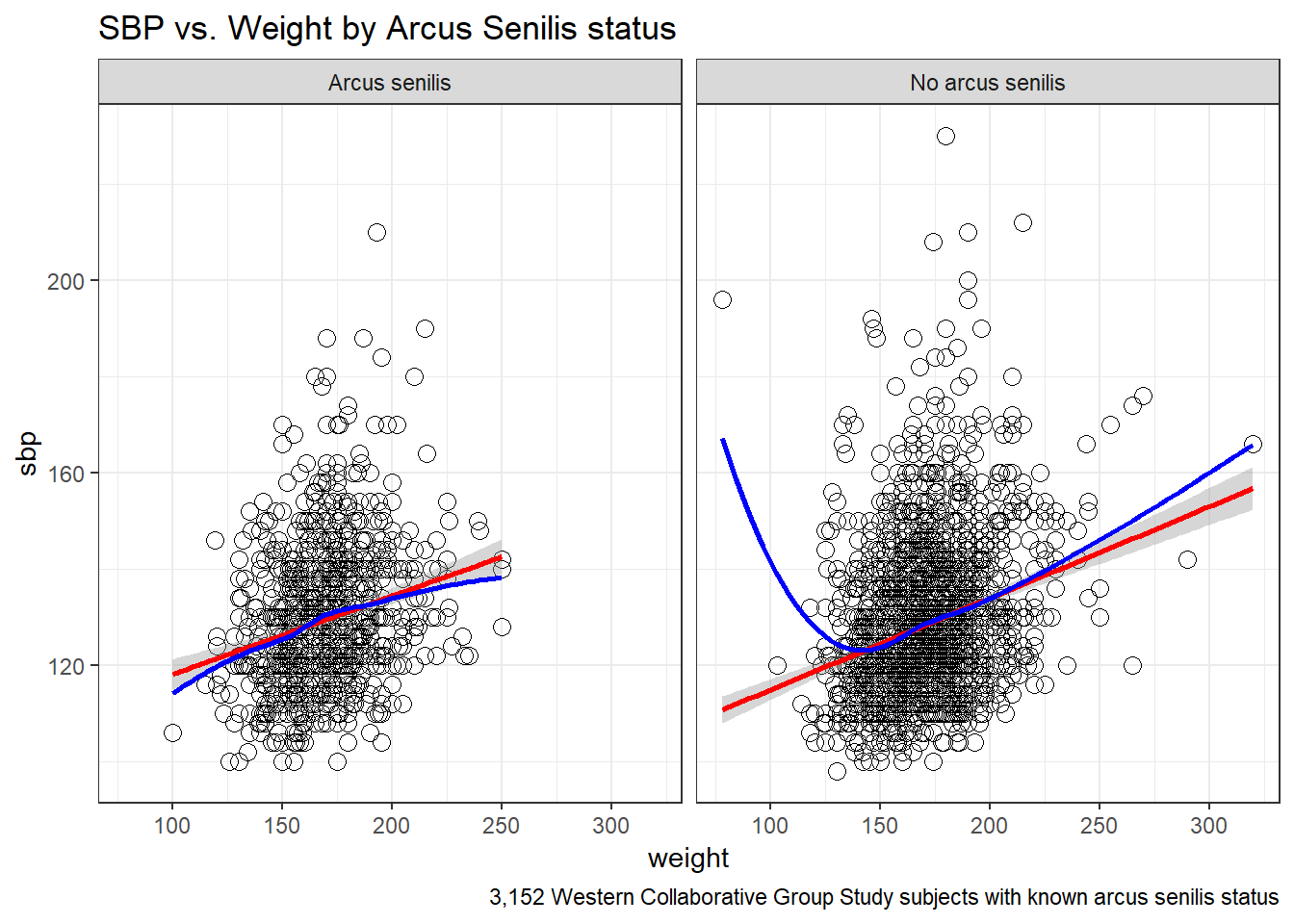
13.8 Linear Model for SBP-Weight Relationship: subjects without Arcus Senilis
Call:
lm(formula = sbp ~ weight, data = filter(wcgs, arcus == 0))

Residuals:
   Min     1Q Median     3Q    Max
-29.01 -10.25  -2.45   7.55  99.85

Coefficients:
            Estimate Std. Error t value Pr(>|t|)
(Intercept)  95.9219     2.5552    37.5   <2e-16 ***
weight        0.1902     0.0149    12.8   <2e-16 ***
---
Signif. codes:  0 '***' 0.001 '**' 0.01 '*' 0.05 '.' 0.1 ' ' 1

Residual standard error: 14.8 on 2209 degrees of freedom
Multiple R-squared:  0.0687,    Adjusted R-squared:  0.0683
F-statistic:  163 on 1 and 2209 DF,  p-value: <2e-16
The linear model for the 2211 patients without Arcus Senilis has R2 = 6.87%.
- The regression equation is 95.92 - 0.19 weight, for those patients without Arcus Senilis.
13.9 Linear Model for SBP-Weight Relationship: subjects with Arcus Senilis
Call:
lm(formula = sbp ~ weight, data = filter(wcgs, arcus == 1))

Residuals:
   Min     1Q Median     3Q    Max
-30.34  -9.64  -1.96   7.97  76.74

Coefficients:
            Estimate Std. Error t value Pr(>|t|)
(Intercept)  101.879      3.756   27.13  < 2e-16 ***
weight         0.163      0.022    7.39  3.3e-13 ***
---
Signif. codes:  0 '***' 0.001 '**' 0.01 '*' 0.05 '.' 0.1 ' ' 1

Residual standard error: 14.2 on 939 degrees of freedom
Multiple R-squared:  0.0549,    Adjusted R-squared:  0.0539
F-statistic: 54.6 on 1 and 939 DF,  p-value: 3.29e-13
The linear model for the 941 patients with Arcus Senilis has R2 = 5.49%.
- The regression equation is 101.88 - 0.163 weight, for those patients with Arcus Senilis.
13.10 Including Arcus Status in the model
Call:
lm(formula = sbp ~ weight * arcus, data = filter(wcgs, !is.na(arcus)))

Residuals:
   Min     1Q Median     3Q    Max
-30.34 -10.15  -2.35   7.67  99.85

Coefficients:
             Estimate Std. Error t value Pr(>|t|)
(Intercept)   95.9219     2.5244   38.00   <2e-16 ***
weight         0.1902     0.0147   12.92   <2e-16 ***
arcus          5.9566     4.6197    1.29     0.20
weight:arcus  -0.0276     0.0270   -1.02     0.31
---
Signif. codes:  0 '***' 0.001 '**' 0.01 '*' 0.05 '.' 0.1 ' ' 1

Residual standard error: 14.6 on 3148 degrees of freedom
Multiple R-squared:  0.066, Adjusted R-squared:  0.0651
F-statistic: 74.1 on 3 and 3148 DF,  p-value: <2e-16
The actual regression equation in this setting includes both weight, and an indicator variable (1 = yes, 0 = no) for arcus senilis status, and the product of weight and that 1/0 indicator.
- Note the use of the product term
weight*arcusin the setup of the model to allow both the slope of weight and the intercept term in the model to change depending on arcus senilis status.- For a patient who has arcus, the regression equation is SBP = 95.92 + 0.19 weight + 5.96 (1) - 0.028 weight (1) = 101.88 + 0.162 weight.
- For a patient without arcus senilis, the regression equation is SBP = 95.92 + 0.19 weight + 5.96 (0) - 0.028 weight (0) = 95.92 + 0.19 weight.
The linear model including the interaction of weight and arcus to predict sbp for the 3152 patients with known Arcus Senilis status has R2 = 6.6%.
13.11 Predictions from these Linear Models
What is our predicted SBP for a subject weighing 175 pounds?
How does that change if our subject weighs 200 pounds?
Recall that
- Without Arcus Senilis, linear model for SBP = 95.9 + 0.19 x weight
- With Arcus Senilis, linear model for SBP = 101.9 + 0.16 x weight
So the predictions for a 175 pound subject are:
95.9 + 0.19 x 175 = 129 mm Hg without Arcus Senilis, and
101.9 + 0.16 x 175 = 130 mm Hg with Arcus Senilis.
And thus, the predictions for a 200 pound subject are:
95.9 + 0.19 x 200 = 134 mm Hg without Arcus Senilis, and
101.9 + 0.16 x 200 = 134.4 mm Hg with Arcus Senilis.
13.12 Scatterplots with Facets Across a Categorical Variable
We can use facets in ggplot2 to show scatterplots across the levels of a categorical variable, like behpat.
ggplot(wcgs, aes(x = weight, y = sbp, col = behpat)) +
    geom_point() +
    facet_wrap(~ behpat) +
    geom_smooth(method = "lm", se = FALSE, col = "black") +
    guides(color = FALSE) +
    theme(strip.text = element_text(face="bold", size=rel(1.25), color="white"),
          strip.background = element_rect(fill="royalblue")) +
    labs(title = "Scatterplots of SBP vs. Weight within Behavior Pattern")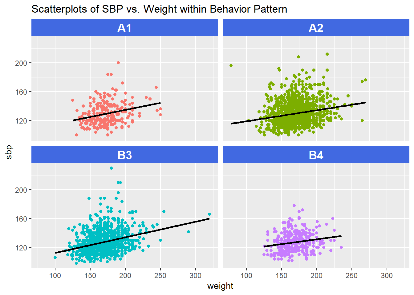
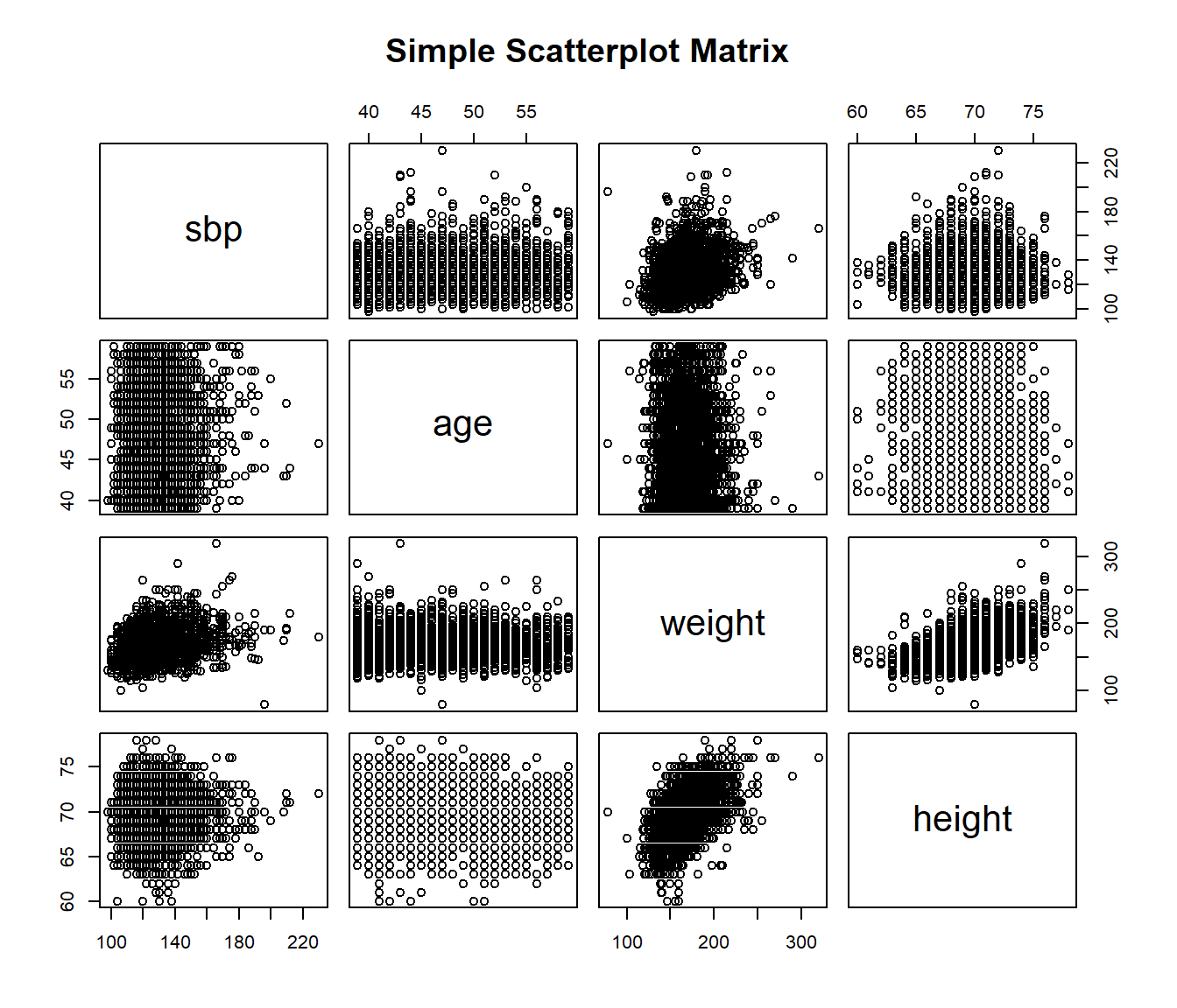
13.13 Scatterplot and Correlation Matrices
A scatterplot matrix can be very helpful in understanding relationships between multiple variables simultaneously. There are several ways to build such a thing, including the pairs function…
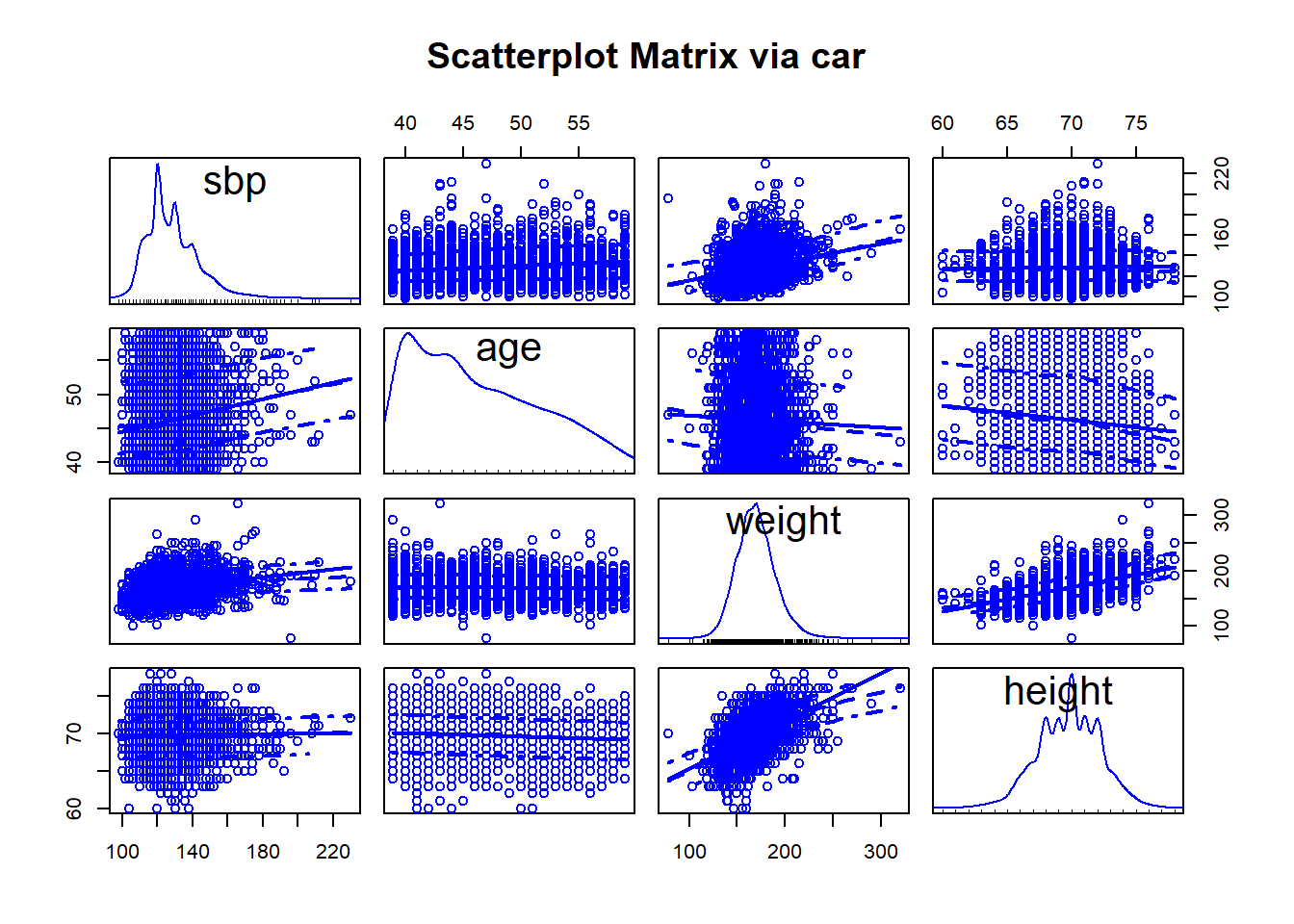
13.13.1 Using the car package
Or, we can use the scatterplotMatrix function from the car package, which adds some detail and fitting to the plots, and places density estimates (with rug plots) on the diagonals.
13.13.2 Displaying a Correlation Matrix
wcgs %>%
    dplyr::select(sbp, age, weight, height) %>%
    cor() %>% # obtain correlation coefficients for this subgroup
    signif(., 3) # round them off to three significant figures before printing
sbp age weight height
sbp 1.0000 0.1660 0.2530 0.0184
age 0.1660 1.0000 -0.0344 -0.0954
weight 0.2530 -0.0344 1.0000 0.5330
height 0.0184 -0.0954 0.5330 1.000013.13.3 Augmented Scatterplot Matrix
Dr. Love’s favorite way to augment a scatterplot matrix adds LOWESS smoothed lines in the upper panel, and correlations in the lower panel, with histograms down the diagonal. To do this, I revised two functions in the Love-boost script (these modifications come from Chang’s R Graphics Cookbook), called panel.hist and panel.cor.
# requires Love-boost.R is sourced

pairs (~ sbp + age + weight + height, data=wcgs,
       main="Augmented Scatterplot Matrix",
       upper.panel = panel.smooth,
       diag.panel = panel.hist,
       lower.panel = panel.cor)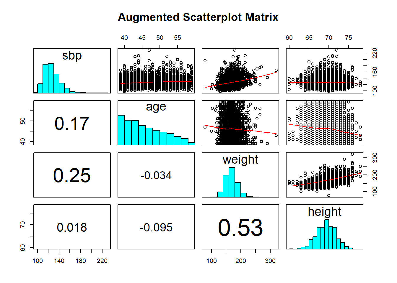
13.13.4 Using the GGally package
The ggplot2 system doesn’t have a built-in scatterplot system. There are some nice add-ins in the world, though. One option I sort of like is in the GGally package, which can produce both correlation matrices and scatterplot matrices.
The ggpairs function provides a density plot on each diagonal, Pearson correlations on the upper right and scatterplots on the lower left of the matrix.
GGally::ggpairs(wcgs %>% select(sbp, age, weight, height),
                title = "Scatterplot Matrix via ggpairs")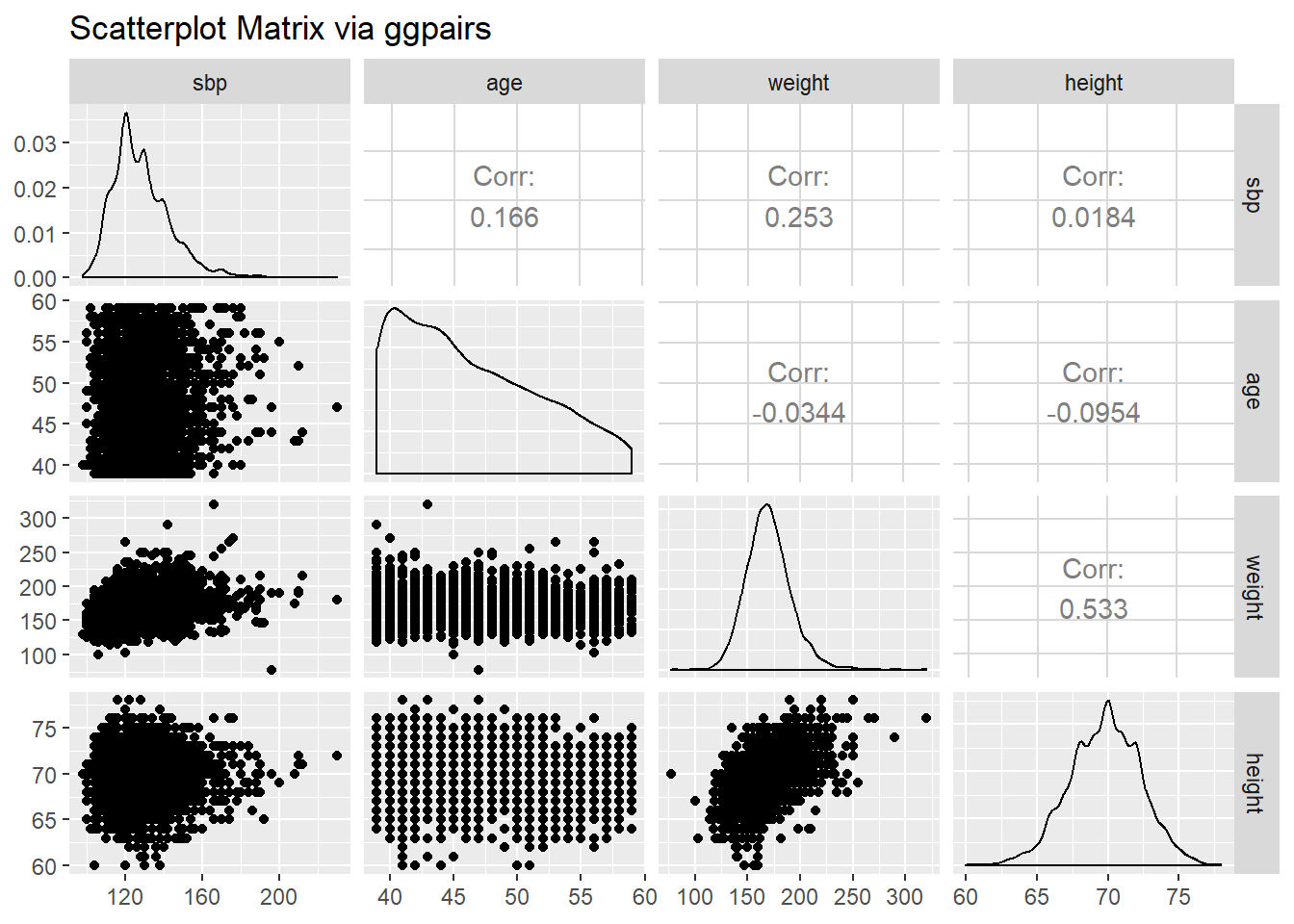
References
Vittinghoff, Eric, David V. Glidden, Stephen C. Shiboski, and Charles E. McCulloch. 2012. Regression Methods in Biostatistics: Linear, Logistic, Survival, and Repeated Measures Models. Second. Springer-Verlag, Inc. http://www.biostat.ucsf.edu/vgsm/.
Grolemund, Garrett, and Hadley Wickham. 2017. R for Data Science. O’Reilly. http://r4ds.had.co.nz/.
For more on the WCGS, you might look at http://www.epi.umn.edu/cvdepi/study-synopsis/western-collaborative-group-study/↩