Chapter 45 BMI and Employment: Working with Categorical Predictors
45.1 The Data
A study recently published in BMJ Open looked at the differential relationship between employment status and body-mass index among middle-aged and elderly adults living in South Korea. Data from this study were available online thanks to the Dryad data package. The original data came from a nationally representative sample of 7228 participants in the Korean Longitudinal Study of Aging. I sampled these data, and did some data “rectangling” (wrangling) to build the emp_bmi.csv file on our web site.
The available data in emp_bmi describe 999 subjects, and included are 8 variables:
| Variable | Description | NA? |
|---|---|---|
pid |
subject identification number (categorical) | 0 |
bmi |
our outcome, quantitative, body-mass index | 0 |
age |
subject’s age (between 51 and 95) | 1 |
gender |
subject’s gender (male or female) | 0 |
employed |
employment status indicator (1/0) | 1 |
married |
marital status indicator (1/0) | 1 |
alcohol |
3-level factor | 2 |
education |
4-level factor | 5 |
emp_bmi

 8  Variables      999  Observations
---------------------------------------------------------------------------
pid
       n  missing distinct     Info     Mean      Gmd      .05      .10
     999        0      999        1    31774    20178     3506     6961
     .25      .50      .75      .90      .95
   16671    31761    46902    54635    58433

lowest :    22    41    52    82   112, highest: 61471 61481 61532 61641 61691
---------------------------------------------------------------------------
bmi
       n  missing distinct     Info     Mean      Gmd      .05      .10
     999        0      373        1    23.24    2.808    19.21    20.13
     .25      .50      .75      .90      .95
   21.54    23.24    24.78    26.56    27.34

lowest : 15.6 15.6 16.2 16.4 16.5, highest: 31.1 31.2 32.0 33.5 34.7
---------------------------------------------------------------------------
age
       n  missing distinct     Info     Mean      Gmd      .05      .10
     998        1       43    0.999    66.29    11.56       52       53
     .25      .50      .75      .90      .95
      57       66       74       81       83

lowest : 51 52 53 54 55, highest: 89 90 92 93 95
---------------------------------------------------------------------------
gender
       n  missing distinct
     999        0        2

Value      female   male
Frequency     570    429
Proportion  0.571  0.429
---------------------------------------------------------------------------
employed
       n  missing distinct     Info      Sum     Mean      Gmd
     998        1        2    0.723      404   0.4048   0.4824

---------------------------------------------------------------------------
married
       n  missing distinct     Info      Sum     Mean      Gmd
     998        1        2    0.548      758   0.7595   0.3657

---------------------------------------------------------------------------
alcohol
       n  missing distinct
     997        2        3

Value                  alcohol dependent                 heavy drinker
Frequency                             45                           306
Proportion                         0.045                         0.307

Value      normal drinker or non-drinker
Frequency                            646
Proportion                         0.648
---------------------------------------------------------------------------
education
       n  missing distinct
     994        5        4

Value      1 elem school grad or lower        2 middle school grad
Frequency                          421                         180
Proportion                       0.424                       0.181

Value               3 high school grad    4 college grad or higher
Frequency                          292                         101
Proportion                       0.294                       0.102
---------------------------------------------------------------------------
45.1.1 Specifying Outcome and Predictors for our Model
In the original study, a key goal was to understand the relationship between employment and body-mass index. Our goal in this example will be to create a model to predict bmi focusing on employment status (so our key predictor is employed) while accounting for the additional predictors age, gender, married, alcohol and education. A natural thing to do would be to consider interactions of these predictor variables (for example, does the relationship between bmi and employed change when comparing men to women?) but we’ll postpone that discussion until 432.
45.1.2 Dealing with Missing Predictor Values
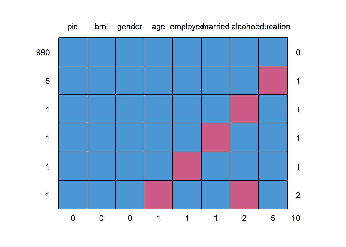
    pid bmi gender age employed married alcohol education
990   1   1      1   1        1       1       1         1  0
5     1   1      1   1        1       1       1         0  1
1     1   1      1   1        1       1       0         1  1
1     1   1      1   1        1       0       1         1  1
1     1   1      1   1        0       1       1         1  1
1     1   1      1   0        1       1       0         1  2
      0   0      0   1        1       1       2         5 10
We will eventually build a model to predict bmi using all of the other variables besides pid. So we’ll eventually have to account for the 9 people with missing values (one of whom has two missing values, as we see above.) What I’m going to do in this example is to first build a complete-case analysis on the 990 subjects without missing values and then, later, do multiple imputation to account for the 9 subjects with missing values (and their 10 actual missing values) sensibly.
I’ll put the “complete cases” data set of 990 subjects in emp_bmi_noNA.
# A tibble: 990 x 8
     pid   bmi   age gender employed married alcohol        education
   <int> <dbl> <int> <fct>     <int>   <int> <fct>          <fct>
 1    22  20.8    58 male          1       1 heavy drinker  4 college gra~
 2    41  21.4    76 female        0       1 normal drinke~ 1 elem school~
 3    52  20.9    66 female        1       1 heavy drinker  1 elem school~
 4    82  23.7    67 male          1       1 alcohol depen~ 2 middle scho~
 5   112  25.5    63 female        0       1 heavy drinker  1 elem school~
 6   181  20.5    51 female        1       1 heavy drinker  3 high school~
 7   182  25.3    51 male          1       1 alcohol depen~ 3 high school~
 8   411  20.8    66 female        1       1 normal drinke~ 2 middle scho~
 9   491  20.8    64 female        0       1 normal drinke~ 3 high school~
10   531  24.3    84 female        0       0 normal drinke~ 1 elem school~
# ... with 980 more rows pid bmi age gender employed married alcohol
0 0 0 0 0 0 0
education
0 45.2 The “Kitchen Sink” Model
A “kitchen sink” model includes all available predictors.
ebmodel.1 <- lm(bmi ~ age + gender + employed + married +
                    alcohol + education, data = emp_bmi_noNA)
summary(ebmodel.1)
Call:
lm(formula = bmi ~ age + gender + employed + married + alcohol +
    education, data = emp_bmi_noNA)

Residuals:
   Min     1Q Median     3Q    Max
-7.703 -1.606 -0.049  1.499 11.730

Coefficients:
                                     Estimate Std. Error t value Pr(>|t|)
(Intercept)                           26.1539     0.8836   29.60  < 2e-16
age                                   -0.0426     0.0107   -4.00  6.9e-05
gendermale                             0.2981     0.2027    1.47    0.142
employed                              -0.4576     0.1915   -2.39    0.017
married                                0.0944     0.2128    0.44    0.657
alcoholheavy drinker                   0.2532     0.4073    0.62    0.534
alcoholnormal drinker or non-drinker   0.1412     0.4077    0.35    0.729
education2 middle school grad         -0.2886     0.2402   -1.20    0.230
education3 high school grad           -0.5012     0.2219   -2.26    0.024
education4 college grad or higher     -0.7986     0.3107   -2.57    0.010

(Intercept)                          ***
age                                  ***
gendermale
employed                             *
married
alcoholheavy drinker
alcoholnormal drinker or non-drinker
education2 middle school grad
education3 high school grad          *
education4 college grad or higher    *
---
Signif. codes:  0 '***' 0.001 '**' 0.01 '*' 0.05 '.' 0.1 ' ' 1

Residual standard error: 2.51 on 980 degrees of freedom
Multiple R-squared:  0.0225,    Adjusted R-squared:  0.0135
F-statistic: 2.51 on 9 and 980 DF,  p-value: 0.00772
45.3 Using Categorical Variables (Factors) as Predictors
We have six predictors here, and five of them are categorical. Note that R recognizes each kind of variable in this case and models them appropriately. Let’s look at the coefficients of our model.
45.3.1 gender: A binary variable represented by letters
The gender variable contains the two categories: male and female, and R recognizes this as a factor. When building a regression model with such a variable, R assigns the first of the two levels of the factor to the baseline, and includes in the model an indicator variable for the second level. By default, R assigns each factor a level order alphabetically.
So, in this case, we have:
[1] TRUE[1] "female" "male" As you see in the model, the gender information is captured by the indicator variable gendermale, which is 1 when gender = male and 0 otherwise.
So, when our model includes:
Coefficients:     Estimate Std. Error t value Pr(>|t|)
gendermale         0.29811    0.20271   1.471   0.1417
this means that a male subject is predicted to have an outcome that is 0.29811 points higher than a female subject, if they have the same values of all of the other predictors.
Note that if we wanted to switch the levels so that “male” came first (and so that R would use “male” as the baseline category and “female” as the 1 value in an indicator), we could do so with the forcats package and the fct_relevel command. Building a model with this version of gender will simply reverse the sign of our indicator variable, but not change any of the other output.
emp_bmi_noNA$gender.2 <- fct_relevel(emp_bmi_noNA$gender, "male", "female")
revised.model <- lm(bmi ~ age + gender.2 + employed + married +
                    alcohol + education, data = emp_bmi_noNA)
summary(revised.model)
Call:
lm(formula = bmi ~ age + gender.2 + employed + married + alcohol +
    education, data = emp_bmi_noNA)

Residuals:
   Min     1Q Median     3Q    Max
-7.703 -1.606 -0.049  1.499 11.730

Coefficients:
                                     Estimate Std. Error t value Pr(>|t|)
(Intercept)                           26.4520     0.9465   27.95  < 2e-16
age                                   -0.0426     0.0107   -4.00  6.9e-05
gender.2female                        -0.2981     0.2027   -1.47    0.142
employed                              -0.4576     0.1915   -2.39    0.017
married                                0.0944     0.2128    0.44    0.657
alcoholheavy drinker                   0.2532     0.4073    0.62    0.534
alcoholnormal drinker or non-drinker   0.1412     0.4077    0.35    0.729
education2 middle school grad         -0.2886     0.2402   -1.20    0.230
education3 high school grad           -0.5012     0.2219   -2.26    0.024
education4 college grad or higher     -0.7986     0.3107   -2.57    0.010

(Intercept)                          ***
age                                  ***
gender.2female
employed                             *
married
alcoholheavy drinker
alcoholnormal drinker or non-drinker
education2 middle school grad
education3 high school grad          *
education4 college grad or higher    *
---
Signif. codes:  0 '***' 0.001 '**' 0.01 '*' 0.05 '.' 0.1 ' ' 1

Residual standard error: 2.51 on 980 degrees of freedom
Multiple R-squared:  0.0225,    Adjusted R-squared:  0.0135
F-statistic: 2.51 on 9 and 980 DF,  p-value: 0.00772
Note that the two categories here need to be both mutually exclusive (a subject cannot be in more than one category) and collectively exhaustive (all subjects must fit into this set of categories) in order to work properly as a regression predictor.
45.3.2 employed: A binary variable represented a 1/0 indicator
The employed and married variables are each described using an indicator variable, which is 1 if the condition of interest holds and 0 if it does not. R doesn’t recognize this as a factor, but rather as a quantitative variable. However, this is no problem for modeling, where we just need to remember that if employed = 1, the subject is employed, and if employed = 0, the subject is not employed, to interpret the results. The same approach is used for married.
Coefficients:    Estimate Std. Error t value Pr(>|t|)
employed         -0.45761    0.19153  -2.389   0.0171 *
married           0.09438    0.21280   0.444   0.6575
So, in our model, if subject A is employed, they are expected to have an outcome that is 0.46 points lower (-0.46 points higher) than subject B who is not employed but otherwise identical to subject A.
Similarly, if subject X is married, and subject Y is unmarried, but they otherwise have the same values of all predictors, then our model will predict a bmi for X that is 0.094 points higher than for Y.
45.3.3 alcohol: A three-category variable coded by names
Our alcohol information divides subjects into three categories, which are:
- normal drinker or non-drinker
- heavy drinker
- alcohol dependent
R builds a model using \(k-1\) predictors to describe a variable with \(k\) levels. As mentioned previously, R selects a baseline category when confronted with a factor variable, and it always selects the first level as the baseline. The levels are sorted alphabetically, unless we tell R to sort them some other way. So, we have
Coefficients:                        Estimate Std. Error t value Pr(>|t|)
alcoholheavy drinker                  0.25317    0.40727   0.622   0.5343
alcoholnormal drinker or non-drinker  0.14121    0.40766   0.346   0.7291
How do we interpret this?
- Suppose subject A is alcohol dependent, B is a heavy drinker and C is a normal drinker or non-drinker, but subjects A-C have the same values of all other predictors.
- Our model predicts that B would have a BMI that is 0.25 points higher than A.
- Our model predicts that C would have a BMI that is 0.14 points higher than A.
A good way to think about this…
| Subject | Status | alcoholheavy drinker | alcoholnormal drinker or non-drinker |
|---|---|---|---|
| A | alcohol dependent | 0 | 0 |
| B | heavy drinker | 1 | 0 |
| C | normal drinker or non-drinker | 0 | 1 |
and so, with two variables, we cover each of these three possible alcohol levels.
When we have an ordered variable like this one, we usually want the baseline category to be at either end of the scale (either the highest or the lowest, but not something in the middle.) Another good idea in many settings is to use as the baseline category the most common category. Here, the baseline R chose was “alcohol dependent” which is the least common category, so I might want to use the fct_relevel function again to force R to choose, say, normal drinker/non-drinker as the baseline category.
emp_bmi_noNA$alcohol.2 <- fct_relevel(emp_bmi_noNA$alcohol,
           "normal drinker or non-drinker", "heavy drinker")
revised.model.2 <- lm(bmi ~ age + gender + employed + married +
                    alcohol.2 + education, data = emp_bmi_noNA)
summary(revised.model.2)
Call:
lm(formula = bmi ~ age + gender + employed + married + alcohol.2 +
    education, data = emp_bmi_noNA)

Residuals:
   Min     1Q Median     3Q    Max
-7.703 -1.606 -0.049  1.499 11.730

Coefficients:
                                  Estimate Std. Error t value Pr(>|t|)
(Intercept)                        26.2951     0.8286   31.73  < 2e-16 ***
age                                -0.0426     0.0107   -4.00  6.9e-05 ***
gendermale                          0.2981     0.2027    1.47    0.142
employed                           -0.4576     0.1915   -2.39    0.017 *
married                             0.0944     0.2128    0.44    0.657
alcohol.2heavy drinker              0.1120     0.1965    0.57    0.569
alcohol.2alcohol dependent         -0.1412     0.4077   -0.35    0.729
education2 middle school grad      -0.2886     0.2402   -1.20    0.230
education3 high school grad        -0.5012     0.2219   -2.26    0.024 *
education4 college grad or higher  -0.7986     0.3107   -2.57    0.010 *
---
Signif. codes:  0 '***' 0.001 '**' 0.01 '*' 0.05 '.' 0.1 ' ' 1

Residual standard error: 2.51 on 980 degrees of freedom
Multiple R-squared:  0.0225,    Adjusted R-squared:  0.0135
F-statistic: 2.51 on 9 and 980 DF,  p-value: 0.00772
How do we interpret this revised model?
- Again, subject A is alcohol dependent, B is a heavy drinker and C is a normal drinker or non-drinker, but subjects A-C have the same values of all other predictors.
- Our model predicts that B would have a BMI that is 0.11 points higher than C.
- Our model predicts that A would have a BMI that is 0.14 points lower than C.
So, those are the same conclusions, just rephrased.
45.3.4 t tests and multi-categorical variables
The usual “last predictor in” t test works perfectly for binary factors, but suppose we have a factor like alcohol which is represented by two different indicator variables. If we want to know whether the alcohol information, as a group, adds statistically significant value to the model that includes all of the other predictors, then our best strategy is to compare two models - one with the alcohol information, and one without.
model.with.a <- lm(bmi ~ age + gender + alcohol + employed + married + education,
                   data = emp_bmi_noNA)
model.no.a <- lm(bmi ~ age + gender + employed + married + education,
                 data = emp_bmi_noNA)
anova(model.with.a, model.no.a)
Analysis of Variance Table
Model 1: bmi ~ age + gender + alcohol + employed + married + education
Model 2: bmi ~ age + gender + employed + married + education
Res.Df RSS Df Sum of Sq F Pr(>F)
1 980 6190
2 982 6194 -2 -3.63 0.29 0.75The p value for both of the indicator variables associated with alcohol combined is 0.75, according to an ANOVA F test with 2 degrees of freedom.
Note that we can get the same information from an ANOVA table of the larger model if we add the alcohol predictor to the model last.
Analysis of Variance Table

Response: bmi
           Df Sum Sq Mean Sq F value Pr(>F)
age         1     56    55.5    8.79 0.0031 **
gender      1      0     0.4    0.06 0.8090
employed    1     31    30.7    4.87 0.0276 *
married     1      0     0.4    0.06 0.8077
education   3     52    17.3    2.74 0.0422 *
alcohol     2      4     1.8    0.29 0.7504
Residuals 980   6190     6.3
---
Signif. codes:  0 '***' 0.001 '**' 0.01 '*' 0.05 '.' 0.1 ' ' 1
Again, we see p for the two alcohol indicators is 0.75.
45.3.5 education: A four-category variable coded by names
The education variable’s codes are a little better designed. By preceding the text with a number for each code, we force R to attend to the level order we want to see.
Coefficients:                     Estimate Std. Error t value Pr(>|t|)
education2 middle school grad     -0.28862    0.24020  -1.202   0.2298
education3 high school grad       -0.50123    0.22192  -2.259   0.0241 *
education4 college grad or higher -0.79862    0.31068  -2.571   0.0103 *
Since we have four education levels, we need those three indicator variables.
education2 middle school gradis 1 if the subject is a middle school graduate, and 0 if they have some other statuseducation3 high school gradis 1 if the subject is a high school graduate, and 0 if they have some other statuseducation4 college grad or higheris 1 if the subject is a college graduate or has more education, and 0 if they have some other status.- So the subjects with only elementary school or lower education are represented by zeros in all three indicators.
Suppose we have four subjects now, with the same values of all other predictors, but different levels of education.
| Subject | Education | Estimated BMI |
|---|---|---|
| A | elementary school or less | A |
| B | middle school grad | A - 0.289 |
| C | high school grad | A - 0.501 |
| D | college grad | A - 0.799 |
Note that the four categories are mutually exclusive (a subject cannot be in more than one category) and collectively exhaustive (all subjects must fit into this set of categories.) As we have seen, this is a requirement of categorical variables in a regression analysis.
Let’s run the ANOVA test for the education information captured in those three indicator variables…
Analysis of Variance Table

Response: bmi
           Df Sum Sq Mean Sq F value Pr(>F)
age         1     56    55.5    8.79 0.0031 **
gender      1      0     0.4    0.06 0.8090
employed    1     31    30.7    4.87 0.0276 *
married     1      0     0.4    0.06 0.8077
alcohol     2      4     1.8    0.28 0.7581
education   3     52    17.4    2.75 0.0418 *
Residuals 980   6190     6.3
---
Signif. codes:  0 '***' 0.001 '**' 0.01 '*' 0.05 '.' 0.1 ' ' 1
So, as a group, the three indicator variables add statistically significant predictive value at the 5% significance level, since the F test for those three variables has p = 0.042
45.3.6 Interpreting the Kitchen Sink Model
So, again, here’s our model, now pandered into a prettier format.
ebmodel.1 <- lm(bmi ~ age + gender + employed + married +
                    alcohol + education, data = emp_bmi_noNA)
pander(ebmodel.1)| Estimate | Std. Error | t value | Pr(>|t|) | |
|---|---|---|---|---|
| (Intercept) | 26.15 | 0.8836 | 29.6 | 4.401e-138 |
| age | -0.0426 | 0.01065 | -3.998 | 6.858e-05 |
| gendermale | 0.2981 | 0.2027 | 1.471 | 0.1417 |
| employed | -0.4576 | 0.1915 | -2.389 | 0.01707 |
| married | 0.09438 | 0.2128 | 0.4435 | 0.6575 |
| alcoholheavy drinker | 0.2532 | 0.4073 | 0.6216 | 0.5343 |
| alcoholnormal drinker or non-drinker | 0.1412 | 0.4077 | 0.3464 | 0.7291 |
| education2 middle school grad | -0.2886 | 0.2402 | -1.202 | 0.2298 |
| education3 high school grad | -0.5012 | 0.2219 | -2.259 | 0.02413 |
| education4 college grad or higher | -0.7986 | 0.3107 | -2.571 | 0.0103 |
If we wanted to predict a BMI level for a new subject like the ones used in the development of this model, that prediction would be:
- 26.15
- minus 0.426 times the subject’s
age - plus 0.298 if the subject’s
genderwasmale - minus 0.458 if the subject’s employment status was
employed - plus 0.253 if the subject’s
alcoholclassification washeavy drinker - plus 0.141 if the subject’s
alcoholclassification wasnormal drinker or non-drinker - minus 0.289 if the subject’s
educationclassification was2 middle school grad - minus 0.501 if the subject’s
educationclassification was3 high school grad - minus 0.799 if the subject’s
educationclassification was4 college grad or higher
45.4 Scatterplot Matrix with Categorical Predictors
Let’s look at a scatterplot matrix of a few key predictors, with my favorite approach (at least for quantitative predictors)…
pairs( ~ bmi + age + gender + employed + education, data = emp_bmi_noNA,
       main = "emp_bmi Scatterplot and Correlation Matrix",
       upper.panel = panel.smooth,
       diag.panel = panel.hist,
       lower.panel = panel.cor)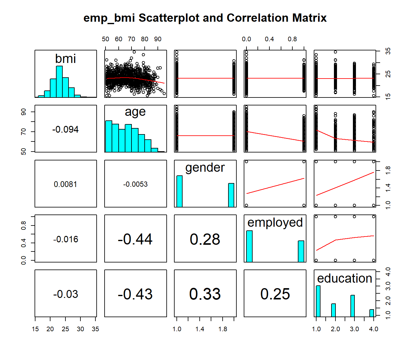
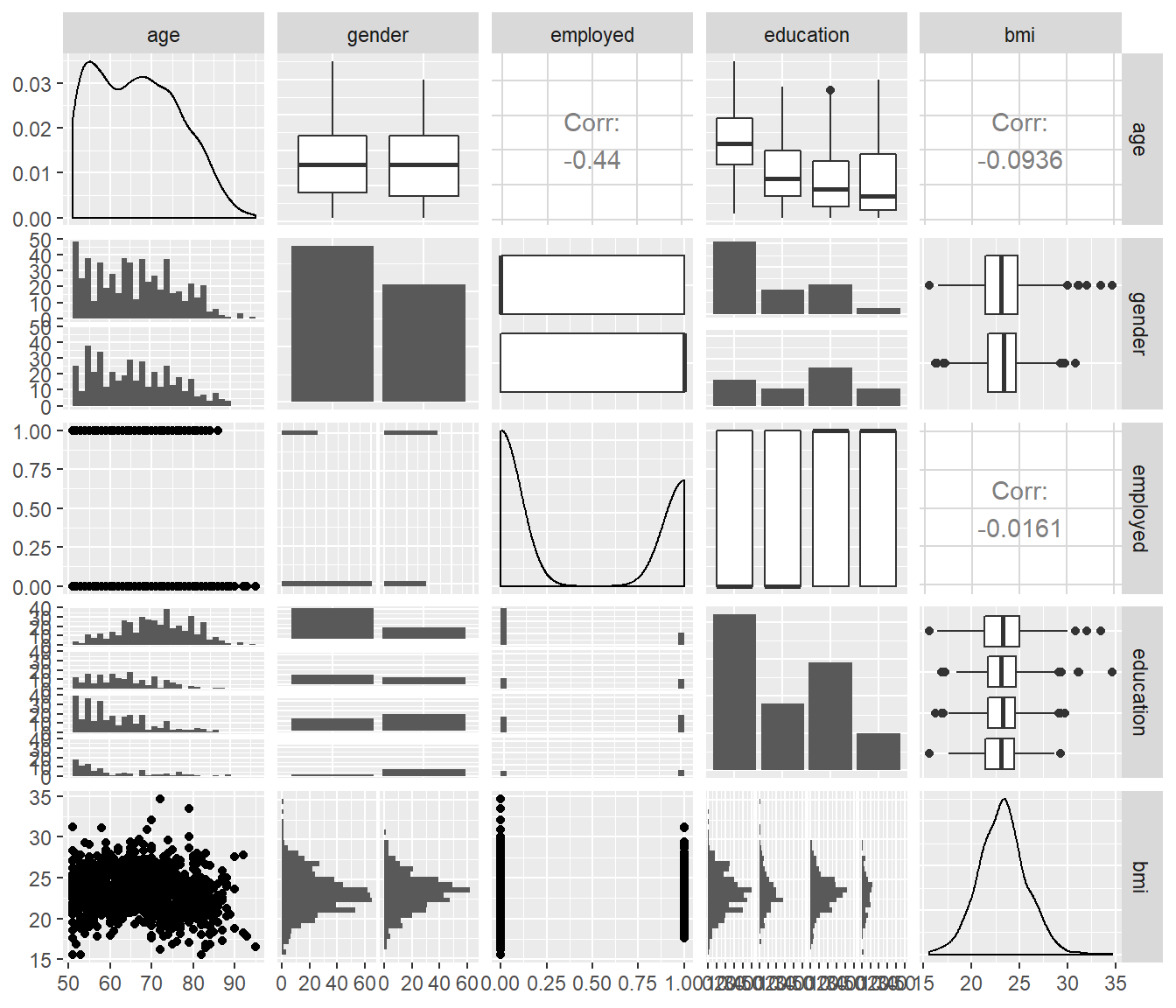
Notice how the ggpairs approach reacts to the inclusion of factors as predictors…
45.5 Residual Plots when we have Categorical Predictors
Here are the main residual plots from the kitchen sink model ebmodel.1 defined previously.
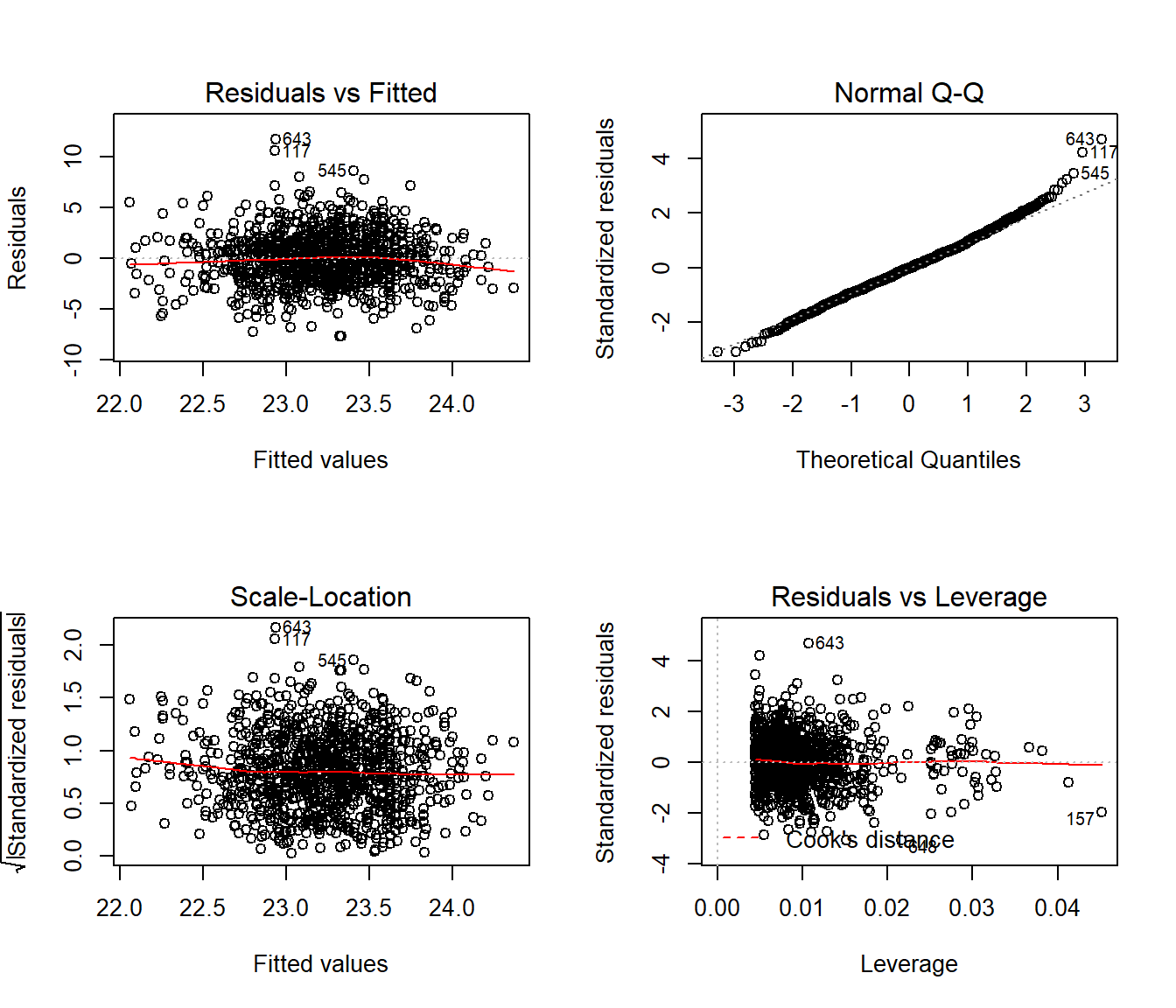
Sometimes, in small samples, the categorical variables will make the regression residuals line up in somewhat strange patterns. But in this case, there’s no real problem. The use of categorical variables also has some impact on leverage, as it’s hard for a subject to be a serious outlier in terms of a predictor if that predictor only has a few possible levels.
45.6 Stepwise Regression and Categorical Predictors
When R does backwards elimination for stepwise model selection, it makes decisions about each categorical variable as in/out across all of the indicator variables simultaneously, as you’d hope.
Start:  AIC=1835
bmi ~ age + gender + employed + married + alcohol + education

            Df Sum of Sq  RSS  AIC
- alcohol    2       3.6 6194 1831
- married    1       1.2 6191 1833
<none>                   6190 1835
- gender     1      13.7 6204 1835
- education  3      52.1 6242 1837
- employed   1      36.1 6226 1838
- age        1     101.0 6291 1849

Step:  AIC=1831
bmi ~ age + gender + employed + married + education

            Df Sum of Sq  RSS  AIC
- married    1       1.0 6195 1829
<none>                   6194 1831
- gender     1      19.1 6213 1832
- education  3      51.9 6245 1833
- employed   1      34.7 6228 1835
- age        1     108.6 6302 1846

Step:  AIC=1829
bmi ~ age + gender + employed + education

            Df Sum of Sq  RSS  AIC
<none>                   6195 1829
- gender     1      22.2 6217 1831
- education  3      51.3 6246 1832
- employed   1      34.4 6229 1833
- age        1     125.4 6320 1847
Call:
lm(formula = bmi ~ age + gender + employed + education, data = emp_bmi_noNA)

Coefficients:
                      (Intercept)                                age
                          26.5021                            -0.0446
                       gendermale                           employed
                           0.3406                            -0.4457
    education2 middle school grad        education3 high school grad
                          -0.2879                            -0.4977
education4 college grad or higher
                          -0.7904
Note that the stepwise approach first drops two degrees of freedom (two indicator variables) for alcohol and then drops the one degree of freedom for married before it settles on a model with age, gender, education and employed.
45.7 Pooling Results after Multiple Imputation
As mentioned earlier, having built a model using complete cases, we should probably investigate the impact of multiple imputation on the missing observations. We’ll fit 100 imputations using the emp_bmi data and then fit a pooled regression model across those imputations.
Now, we’ll fit the pooled kitchen sink regression model to these imputed data sets and pool them.
model.empbmi.mi <- with(emp_bmi_mi, lm(bmi ~ age + gender + employed + married +
                          alcohol + education))
round(summary(pool(model.empbmi.mi)),3)
estimate std.error statistic df
(Intercept) 26.125 0.878 29.766 985
age -0.042 0.011 -3.977 985
gendermale 0.298 0.202 1.480 986
employed -0.464 0.190 -2.441 987
married 0.097 0.212 0.458 987
alcoholheavy drinker 0.259 0.402 0.645 987
alcoholnormal drinker or non-drinker 0.143 0.403 0.356 987
education2 middle school grad -0.271 0.239 -1.134 983
education3 high school grad -0.500 0.221 -2.262 981
education4 college grad or higher -0.796 0.309 -2.578 983
p.value
(Intercept) 0.000
age 0.000
gendermale 0.139
employed 0.015
married 0.647
alcoholheavy drinker 0.519
alcoholnormal drinker or non-drinker 0.722
education2 middle school grad 0.257
education3 high school grad 0.024
education4 college grad or higher 0.010Note that in summarizing these pooled results, R does some strange things:
- it relabels the indicator variables as
gender2rather thangendermaleso you need to know the level order for each variable. - it leaves as NA the number of missing values imputed for every categorical variable it recognizes as a factor.