Chapter 40 Simple Regression: Using Dose to predict Recovery

To start, consider a simple (one predictor) regression model using dose alone to predict the % Recovery (recov.score). Ignoring the age and weight covariates, what can we conclude about this relationship?

40.1 The Scatterplot, with fitted Linear Model

ggplot(hydrate, aes(x = dose, y = recov.score)) +
    geom_point(size = 2) +
    geom_smooth(method = "lm", col = "red") +
    theme_bw() +
    labs(title = "Simple Regression model for the hydrate data",
         x = "Dose (mEq/l)", y = "Recovery Score (points)")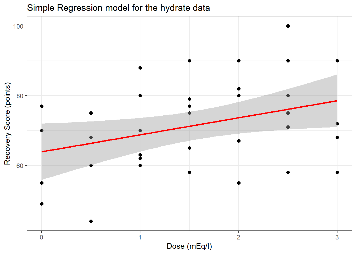

40.2 The Fitted Linear Model

To obtain the fitted linear regression model, we use the lm function:

lm(recov.score ~ dose, data = hydrate)


Call:
lm(formula = recov.score ~ dose, data = hydrate)

Coefficients:
(Intercept)         dose  
      63.90         4.88

So, our fitted regression model (prediction model) is recov.score = 63.9 + 4.88 dose.

40.2.1 Confidence Intervals

We can obtain confidence intervals around the coefficients of our fitted model using the confint function.

confint(lm(recov.score ~ dose, data = hydrate))

             2.5 % 97.5 %
(Intercept) 55.827   72.0
dose         0.466    9.3

40.3 The Summary Output

To get a more complete understanding of the fitted model, we’ll summarize it.

summary(lm(recov.score ~ dose, data = hydrate))


Call:
lm(formula = recov.score ~ dose, data = hydrate)

Residuals:
    Min      1Q  Median      3Q     Max 
-22.336  -7.276   0.063   8.423  23.903 

Coefficients:
            Estimate Std. Error t value Pr(>|t|)    
(Intercept)    63.90       3.97   16.09   <2e-16 ***
dose            4.88       2.17    2.25    0.031 *  
---
Signif. codes:  0 '***' 0.001 '**' 0.01 '*' 0.05 '.' 0.1 ' ' 1

Residual standard error: 12.2 on 34 degrees of freedom
Multiple R-squared:  0.129, Adjusted R-squared:  0.104 
F-statistic: 5.05 on 1 and 34 DF,  p-value: 0.0313

40.3.1 Model Specification

The first part of the output specifies the model that has been fit.
- Here, we have a simple regression model that predicts recov.score on the basis of dose.
- Notice that we’re treating dose here as a quantitative variable. If we wanted dose to be treated as a factor, we’d have specified that in the model.

40.3.2 Residual Summary

The second part of the output summarizes the regression residuals across the subjects involved in fitting the model.
- The residual is defined as the Actual value of our outcome minus the predicted value of that outcome fitted by the model.
- In our case, the residual for a given child is their actual recov.score minus the predicted recov.score according to our model, for that child.
- The residual summary gives us a sense of how “incorrect” our predictions are for the hydrate observations.
  - A positive residual means that the observed value was higher than the predicted value from the linear regression model, so the prediction was too low.
  - A negative residual means that the observed value was lower than the predicted value from the linear regression model, so the prediction was too high.
  - The residuals will center near 0 (the ordinary least squares model fitting process is designed so the mean of the residuals will always be zero)
  - We hope to see the median of the residuals also be near zero, generally. In this case, the median prediction is 0.06 point too low.
  - The minimum and maximum show us the largest prediction errors, made in the subjects used to fit this model.
  - Here, we predicted a recovery score that was 22.3 points too high for one patient, and another of our predicted recovery scores was 23.9 points too low.
  - The middle half of our predictions were between 8.4 points too low and 7.3 points too high.

40.3.3 Coefficients Output

The Coefficients output begins with a table of the estimated coefficients from the regression equation.
- Generally, we write a simple regression model as \(y = \beta_0 + \beta_1 x\).
- In the hydrate model, we have recov.score = \(\beta_0\) + \(\beta_1\) dose.
- The first column of the table gives the estimated \(\beta\) coefficients for our model
  - Here the estimated intercept \(\hat{\beta_0} = 63.9\)
  - The estimated slope of dose \(\hat{\beta_1} = 4.88\)
  - Thus, our model is recov.score= 63.9 + 4.88 dose

We interpret these coefficients as follows:

The intercept (63.9) is the predicted recov.score for a patient receiving a dose of 0 mEq/l of the electrolytic solution.
The slope (4.88) of the dose is the predicted change in recov.score associated with a 1 mEq/l increase in the dose of electrolytic solution.
- Essentially, if we have two children like the ones studied here, and we give Roger a popsicle with dose X and Sarah a popsicle with dose X + 1, then this model predicts that Sarah will have a recovery score that is 4.88 points higher than will Roger.
- From the confidence interval output we saw previously with the function confint(lm(recov.score ~ dose)), we are 95% confident that the true slope for dose is between (0.47, 9.30) mEq/l. We are also 95% confident that the true intercept is between (55.8, 72.0).

40.3.4 Correlation and Slope

If we like, we can use the cor function to specify the Pearson correlation of recov.score and dose, which turns out to be 0.36. - Note that the slope in a simple regression model will follow the sign of the Pearson correlation coefficient, in this case, both will be positive.

cor(hydrate$recov.score, hydrate$dose)

[1] 0.36

40.3.5 Coefficient Testing

summary(lm(recov.score ~ dose, data = hydrate))


Call:
lm(formula = recov.score ~ dose, data = hydrate)

Residuals:
    Min      1Q  Median      3Q     Max 
-22.336  -7.276   0.063   8.423  23.903 

Coefficients:
            Estimate Std. Error t value Pr(>|t|)    
(Intercept)    63.90       3.97   16.09   <2e-16 ***
dose            4.88       2.17    2.25    0.031 *  
---
Signif. codes:  0 '***' 0.001 '**' 0.01 '*' 0.05 '.' 0.1 ' ' 1

Residual standard error: 12.2 on 34 degrees of freedom
Multiple R-squared:  0.129, Adjusted R-squared:  0.104 
F-statistic: 5.05 on 1 and 34 DF,  p-value: 0.0313

Next to each coefficient in the summary regression table is its estimated standard error, followed by the coefficient’s t value (the coefficient value divided by the standard error), and the associated two-tailed p value for the test of:

H₀: This coefficient’s \(\beta\) value = 0 vs.
H_A: This coefficient’s \(\beta\) value \(\neq\) 0.

For the slope coefficient, we can interpret this choice as:

H₀: This predictor adds no predictive value to the model vs.
H_A: This predictor adds statistically significant predictive value to the model.

The t test of the intercept is rarely of interest, because a. we rarely care about the situation that the intercept predicts, where all of the predictor variables are equal to zero and b. we usually are going to keep the intercept in the model regardless of its statistical significance.

In the hydrate simple regression model,

the intercept is statistically significantly different from zero at all reasonable \(\alpha\) levels since Pr(>|t|), the p value is (for all intents and purposes) zero.
A significant p value for this intercept implies that the predicted recovery score for a patient fed a popsicle with 0 mEq/l of the electrolytic solution will be different than 0%.
By running the confint function we have previously seen, we can establish a confidence interval for the intercept term (and the slope of dose, as well).

confint(lm(recov.score ~ dose, data = hydrate), level = .95)

             2.5 % 97.5 %
(Intercept) 55.827   72.0
dose         0.466    9.3

The t test for the slope of dose, on the other hand, is important. This tests the hypothesis that the true slope of dose is zero vs. a two-tailed alternative.

If the slope of dose was in fact zero, then this would mean that knowing the dose information would be of no additional value in predicting the outcome over just guessing the mean of recov.score for every subject.

So, since the slope of dose is significantly different than zero (as it is at the 5% significance level, since p = 0.031),

dose has statistically significant predictive value for recov.score,
more generally, this model has statistically significant predictive value as compared to a model that ignores the dose information and simply predicts the mean of recov.score for each subject.

40.3.6 Summarizing the Quality of Fit

The next part of the regression summary output is a summary of fit quality.

The residual standard error estimates the standard deviation of the prediction errors made by the model.

If assumptions hold, the model will produce residuals that follow a Normal distribution with mean 0 and standard deviation equal to this residual standard error.
- So we’d expect roughly 95% of our residuals to fall between -2(12.21) and +2(12.21), or roughly -24.4 to +24.4 and that we’d see virtually no residuals outside the range of -3(12.21) to +3(12.21), or roughly -36.6 to +36.6.
- The output at the top of the summary tells us about the observed regression residuals, and that they actually range from -22 to +24.
- In context, it’s hard to know whether or not we should be happy about this. On a scale from 0 to 100, rarely missing by more than 24 seems OK to me, but not terrific.
The degrees of freedom here are the same as the denominator degrees of freedom in the ANOVA to follow. The calculation is \(n - k\), where \(n\) = the number of observations and \(k\) is the number of coefficients estimated by the regression (including the intercept and any slopes).
- Here, there are 36 observations in the model, and we fit k = 2 coefficients; the slope and the intercept, as in any simple regression model, so df = 36 - 2 = 34.

The multiple R² value is usually just referred to as R² or R-squared.

This is interpreted as the proportion of variation in the outcome variable that has been accounted for by our regression model.
- Here, we’ve accounted for just under 13% of the variation in % Recovery using Dose.
The R in multiple R-squared is the Pearson correlation of recov.score and dose, which in this case is 0.3595.
- Squaring this value gives the R² for this simple regression.
- (0.3595)^2 = 0.129

R² is greedy.

R² will always suggest that we make our models as big as possible, often including variables of dubious predictive value.
As a result, there are various methods for adjusting or penalizing R² so that we wind up with smaller models.
The adjusted R² is often a useful way to compare multiple models for the same response.
- \(R^2_{adj} = 1 - \frac{(1-R^2)(n - 1)}{n - k}\), where \(n\) = the number of observations and \(k\) is the number of coefficients estimated by the regression (including the intercept and any slopes).
- So, in this case, \(R^2_{adj} = 1 - \frac{(1 - 0.1293)(35)}{34} = 0.1037\)
- The adjusted R² value is not, technically, a proportion of anything, but it is comparable across models for the same outcome.
- The adjusted R² will always be less than the (unadjusted) R².

40.3.7 ANOVA F test

The last part of the standard summary of a regression model is the overall ANOVA F test.

The hypotheses for this test are:

H₀: The model has no statistically significant predictive value, at all vs.
H_A: The model has statistically significant predictive value.

This is equivalent to:

H₀: Each of the coefficients in the model (other than the intercept) has \(\beta\) = 0 vs.
H_A: At least one regression slope has \(\beta \neq\) 0

Since we are doing a simple regression with just one predictor, the ANOVA F test hypotheses are exactly the same as the t test for dose:

H₀: The slope for dose has \(\beta\) = 0 vs.
H_A: The slope for dose has \(\beta \neq\) 0

In this case, we have an F statistic of 5.05 on 1 and 34 degrees of freedom, yielding p = 0.03

At \(\alpha = 0.05\), we conclude that there is statistically significant predictive value somewhere in this model, since p < 0.05.
- This is conclusive evidence that “something” in our model (here, dose is the only predictor) predicts the outcome to a degree beyond that easily attributed to chance alone.
Another appropriate conclusion is that the R² value (13%) is a statistically significant amount of variation in recov.score that is accounted for by a linear regression on dose.
In simple regression (regression with only one predictor), the t test for the slope (dose) always provides the same p value as the ANOVA F test.
- The F test statistic in a simple regression is always by definition just the square of the slope’s t test statistic.
- Here, F = 5.047, and this is the square of t = 2.247 from the Coefficients output

40.4 Viewing the complete ANOVA table

We can obtain the complete ANOVA table associated with this particular model, and the details behind this F test using the anova function:

anova(lm(recov.score ~ dose, data = hydrate))

Analysis of Variance Table

Response: recov.score
          Df Sum Sq Mean Sq F value Pr(>F)  
dose       1    752     752    5.05  0.031 *
Residuals 34   5067     149                 
---
Signif. codes:  0 '***' 0.001 '**' 0.01 '*' 0.05 '.' 0.1 ' ' 1

The R² for our regression model is equal to the \(\eta^2\) for this ANOVA model.
- If we divide SS(dose) = 752.2 by the total sum of squares (752.2 + 5066.7), we’ll get the multiple R² [0.1293]
Note that this is not the same ANOVA model we would get if we treated dose as a factor with seven levels, rather than as a quantitative variable.

40.5 Plotting Residuals vs. Fitted Values

We can obtain the plot of residuals vs. fitted values from this model using:

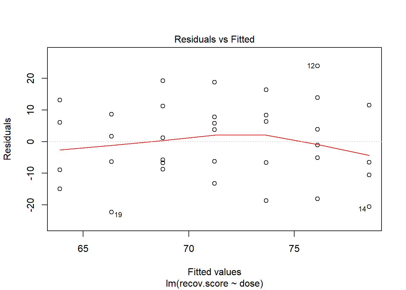
plot(lm(recov.score ~ dose, data = hydrate), which = 1)

We hope in this plot to see a generally random scatter of points, perhaps looking like a “fuzzy football”. Since we only have seven possible dose values, we obtain only seven distinct predicted values, which explains the seven vertical lines in the plot. Here, the smooth red line indicates a gentle curve, but no evidence of a strong curve, or any other regular pattern in this residual plot.

To save the residuals and predicted (fitted) values from this simple regression model, we can use the resid and fitted commands, respectively, or we can use the augment function in the broom package to obtain a tidy data set containing these objects and others.