19 Two Factor ANOVA
19.1 R setup for this chapter
Note
Appendix A lists all R packages used in this book, and also provides R session information. Appendix B describes the 431-Love.R script, and demonstrates its use.
19.2 Data are Rosner’s FEV Data
Note
Appendix C provides further guidance on pulling data from other systems into R, while Appendix D gives more information (including download links) for all data sets used in this book.
Rosner’s FEV data in https://hbiostat.org/data/ FEV (quant) as a function of age, height, sex, smoker should be useful for a two-way anova perhaps adjusting for two additional continuous covariates
fev_ros <- read_csv("data/fev_ros.csv", show_col_types = FALSE) |>
  mutate(across(where(is.character), as_factor)) |>
  mutate(id = as.character(id))

fev_ros
# A tibble: 654 × 6
id age fev height sex smoke
<chr> <dbl> <dbl> <dbl> <fct> <fct>
1 301 9 1.71 57 female non-current smoker
2 451 8 1.72 67.5 female non-current smoker
3 501 7 1.72 54.5 female non-current smoker
4 642 9 1.56 53 male non-current smoker
5 901 9 1.90 57 male non-current smoker
6 1701 8 2.34 61 female non-current smoker
7 1752 6 1.92 58 female non-current smoker
8 1753 6 1.42 56 female non-current smoker
9 1901 8 1.99 58.5 female non-current smoker
10 1951 9 1.94 60 female non-current smoker
# ℹ 644 more rowsn_miss(fev_ros)[1] 019.3 Interaction Plot
19.3.1 Simple Plot of Means
fev_ros |> group_by(sex, smoke) |>
  summarise(mean_fev = mean(fev)) |>
  ggplot(aes(x = sex, y = mean_fev, group = smoke, col = smoke)) +
  geom_point() +
  geom_line() +
  scale_color_metro_d() +
  labs(x = "sex", y = "Mean of FEV")
`summarise()` has grouped output by 'sex'. You can override using the `.groups`
argument.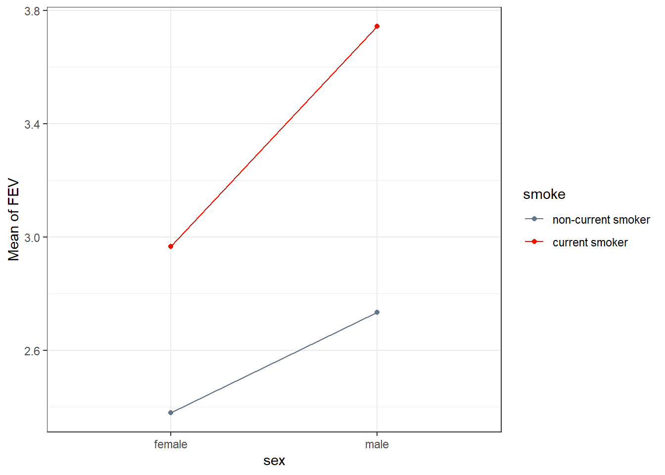
19.3.2 Labeled Interaction Plot
fev_ros |> group_by(sex, smoke) |>
  summarise(mean_fev = mean(fev)) |>
  ggplot(aes(x = smoke, y = mean_fev, group = sex, col = sex)) +
  geom_line() +
  geom_label(aes(label = round(mean_fev,2))) +
  scale_color_see_d() +
  labs(x = "Smoking Status", y = "Mean of FEV",
       title = "Interaction of Sex and Smoking Status on Mean of FEV",
       subtitle = "Rosner data")
`summarise()` has grouped output by 'sex'. You can override using the `.groups`
argument.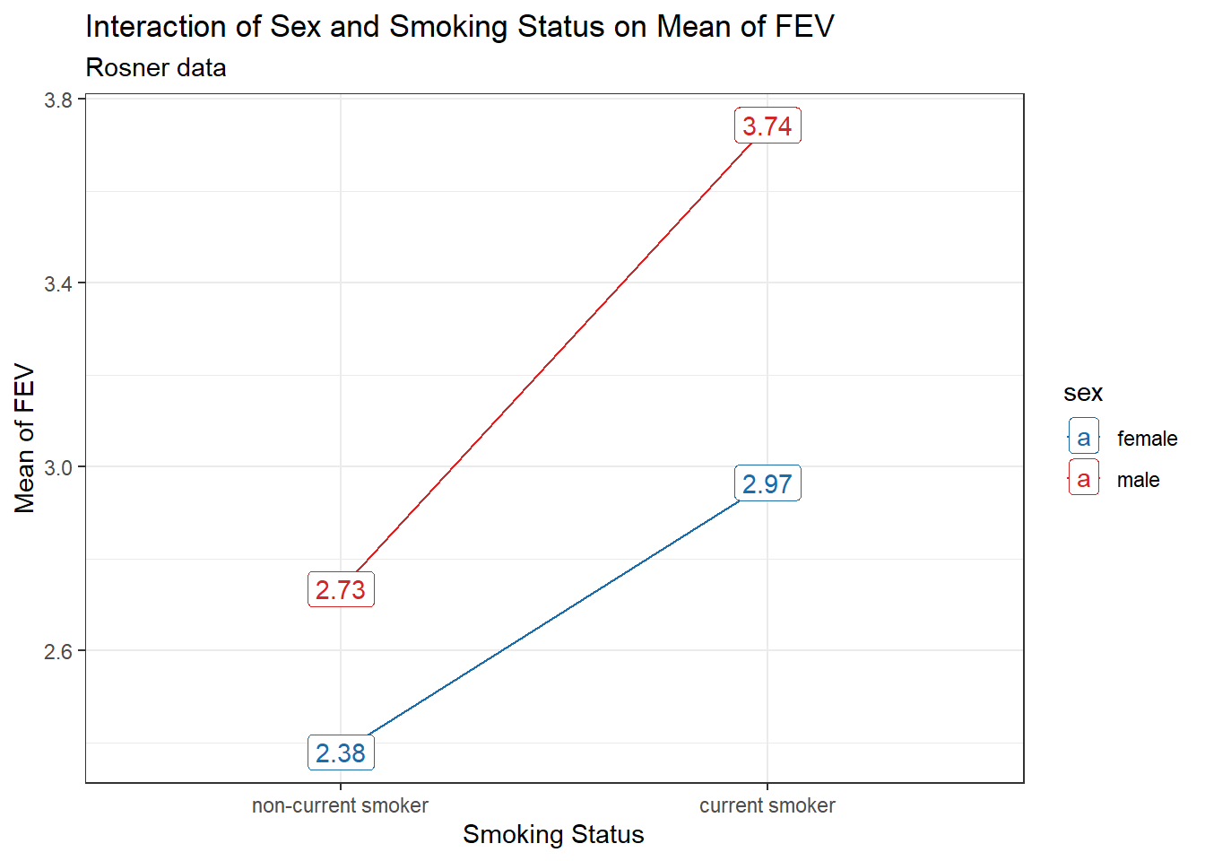
19.4 ANOVA models
fit1 <- aov(fev ~ sex * smoke, data = fev_ros)

model_parameters(fit1, es_type = "eta", ci = 0.95)
Parameter | Sum_Squares | df | Mean_Square | F | p | Eta2 (partial) | Eta2 95% CI
--------------------------------------------------------------------------------------------
sex | 21.32 | 1 | 21.32 | 31.98 | < .001 | 0.05 | [0.02, 1.00]
smoke | 33.68 | 1 | 33.68 | 50.51 | < .001 | 0.07 | [0.04, 1.00]
sex:smoke | 2.51 | 1 | 2.51 | 3.77 | 0.053 | 5.76e-03 | [0.00, 1.00]
Residuals | 433.40 | 650 | 0.67 | | | |
Anova Table (Type 1 tests)fit2 <- lm(fev ~ sex * smoke, data = fev_ros)
model_parameters(fit2, ci = 0.95)Parameter | Coefficient | SE | 95% CI | t(650) | p
------------------------------------------------------------------------------------------
(Intercept) | 2.38 | 0.05 | [ 2.28, 2.48] | 48.67 | < .001
sex [male] | 0.36 | 0.07 | [ 0.22, 0.49] | 5.27 | < .001
smoke [current smoker] | 0.59 | 0.14 | [ 0.31, 0.86] | 4.20 | < .001
sex [male] × smoke [current smoker] | 0.42 | 0.22 | [ 0.00, 0.85] | 1.94 | 0.053
Uncertainty intervals (equal-tailed) and p-values (two-tailed) computed
  using a Wald t-distribution approximation.
19.4.1 Bootstrapping CIs for estimates
set.seed(431)
model_parameters(fit2,
           ci = 0.95, ci_method = "quantile",
           bootstrap = TRUE, iteractions = 1000)
Parameter | Coefficient | 95% CI | p
--------------------------------------------------------------------------
(Intercept) | 2.38 | [ 2.31, 2.45] | < .001
sex [male] | 0.35 | [ 0.22, 0.49] | < .001
smoke [current smoker] | 0.58 | [ 0.44, 0.73] | < .001
sex [male] × smoke [current smoker] | 0.43 | [-0.01, 0.81] | 0.052
Uncertainty intervals (equal-tailed) are naıve bootstrap intervals.19.5 ANOVA without interaction
fit3 <- aov(fev ~ sex + smoke, data = fev_ros)

model_parameters(fit3, es_type = "eta", ci = 0.95)
Parameter | Sum_Squares | df | Mean_Square | F | p | Eta2 (partial) | Eta2 95% CI
--------------------------------------------------------------------------------------------
sex | 21.32 | 1 | 21.32 | 31.85 | < .001 | 0.05 | [0.02, 1.00]
smoke | 33.68 | 1 | 33.68 | 50.30 | < .001 | 0.07 | [0.04, 1.00]
Residuals | 435.91 | 651 | 0.67 | | | |
Anova Table (Type 1 tests)anova(fit3, fit1)Analysis of Variance Table
Model 1: fev ~ sex + smoke
Model 2: fev ~ sex * smoke
Res.Df RSS Df Sum of Sq F Pr(>F)
1 651 435.91
2 650 433.40 1 2.5127 3.7684 0.05266 .
---
Signif. codes: 0 '***' 0.001 '**' 0.01 '*' 0.05 '.' 0.1 ' ' 119.6 Considering Model Diagnostics
check_model(fit1)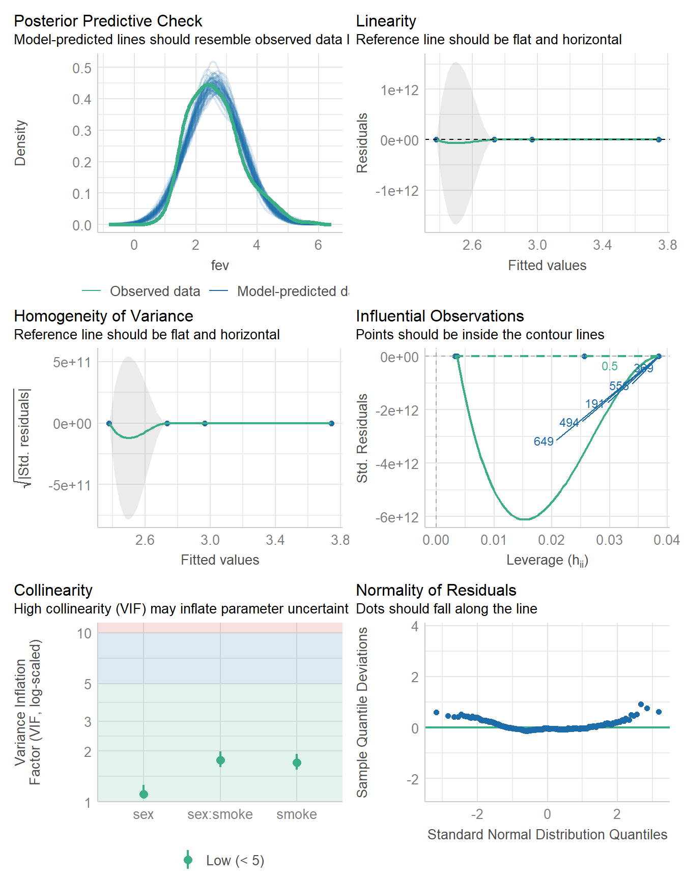
check_model(fit3)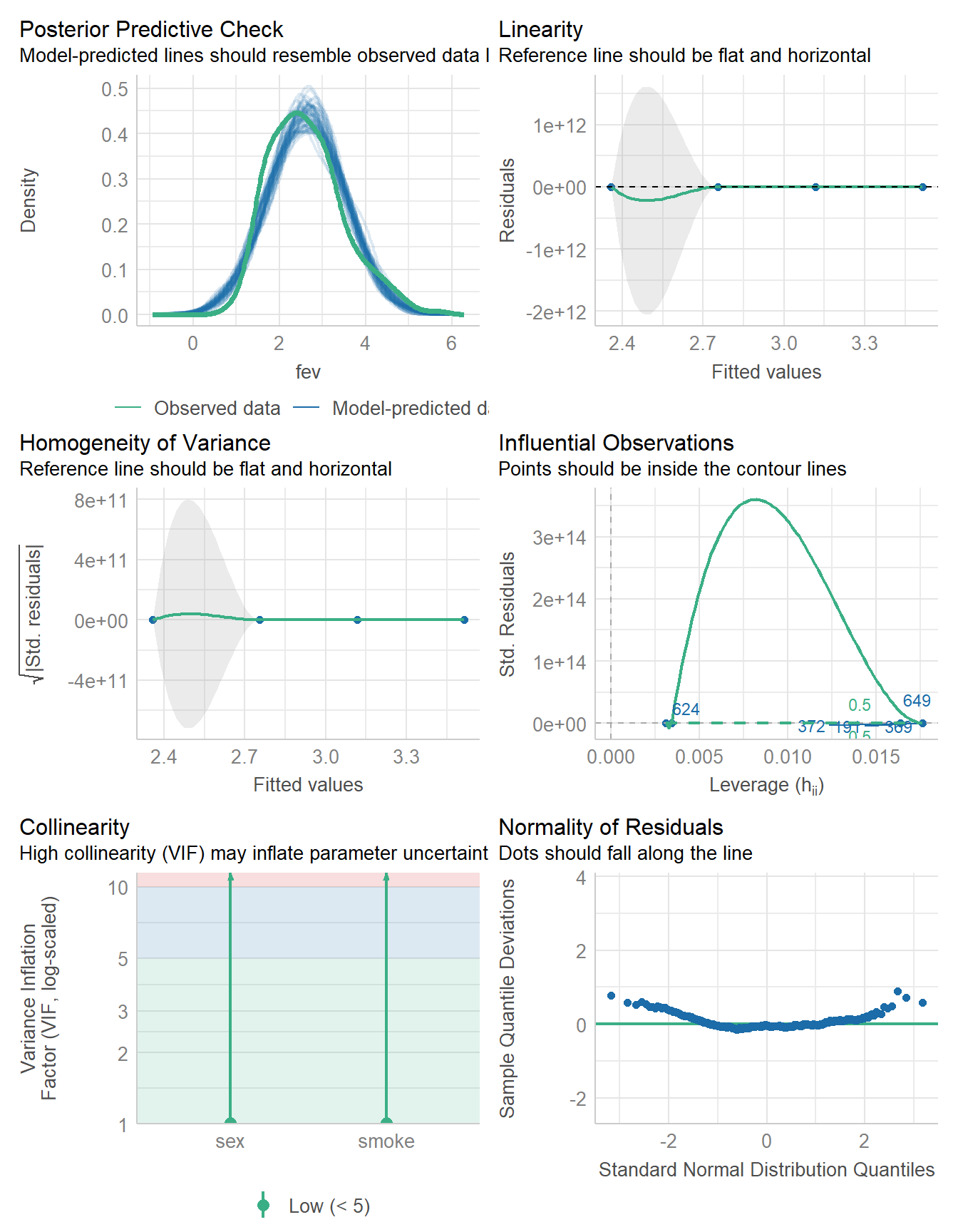
19.7 Comparing Model Performance
compare_performance(fit1, fit3)# Comparison of Model Performance Indices
Name | Model | AIC (weights) | AICc (weights) | BIC (weights) | R2 | R2 (adj.) | RMSE | Sigma
---------------------------------------------------------------------------------------------------
fit1 | aov | 1596.9 (0.709) | 1597.0 (0.706) | 1619.3 (0.206) | 0.117 | 0.113 | 0.814 | 0.817
fit3 | aov | 1598.7 (0.291) | 1598.7 (0.294) | 1616.6 (0.794) | 0.112 | 0.109 | 0.816 | 0.818plot(compare_performance(fit1, fit3))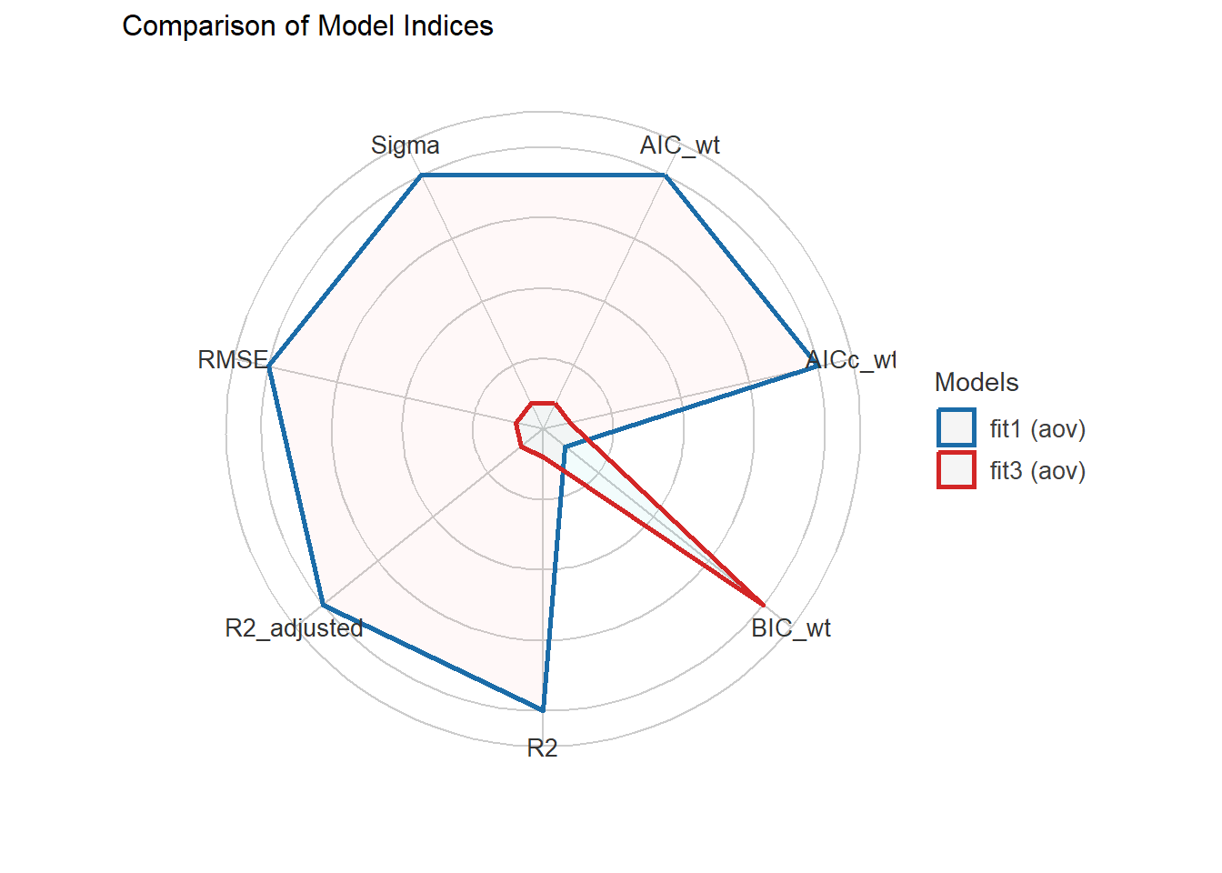
19.8 For More Information
- Class 18 (2024-10-29) contains a lot of additional information about the topics in this chapter. See the slides for that class for more details, please.