10  Storing Blood

10.1 R setup for this chapter

Note

Appendix A lists all R packages used in this book, and also provides R session information. Appendix B describes the 431-Love.R script, and demonstrates its use.

library(car)
library(ggdist)
library(janitor)
library(knitr)
library(naniar)
library(patchwork)
library(rstanarm)

library(easystats)
library(tidyverse)

source("data/Love-431.R")
theme_set(theme_bw())

10.2 Blood Storage data

Note

Appendix C provides further guidance on pulling data from other systems into R, while Appendix D gives more information (including download links) for all data sets used in this book.

The storage.Rds tibble we provide comes from the Cleveland Clinic Statistical Dataset Repository. The source¹ is Cata, Klein, and al. (2011). A version of the data is also available as part of the medicaldata package in R (see Higgins (2023).)

From the CCF Repository, we have the following background:

In cancer patients, perioperative blood transfusion has long been suspected of reducing long-term survival, but available evidence is inconsistent. An important factor associated with the deleterious effects of blood transfusion is the storage age of the transfused blood units. It is suspected that cancer recurrence may be worsened after the transfusion of older blood.

This study evaluated the association between red blood cells (RBC) storage duration and biochemical prostate cancer recurrence after radical prostatectomy. Specifically, tested was the hypothesis that perioperative transfusion of allogeneic RBCs stored for a prolonged period is associated with earlier biochemical recurrence of prostate cancer after prostatectomy.

Patients were assigned to 1 of 3 RBC age exposure groups on the basis of the terciles (ie, the 33rd and 66th percentiles) of the overall distribution of RBC storage duration if all their transfused units could be loosely characterized as of “younger,” “middle,” or “older” age.

The sample we study here includes data on 307 men who:

• had undergone radical prostatectomy and
• received transfusion during or within 30 days of the surgical procedure at Cleveland Clinic and
• had available PSA follow-up data, and
• who received solely allogeneic blood products (rather than a combination) and could be classified into one of the three RBC age exposure groups, and
• did not have any missing data on prostate volume.

The variable we’ll study here is the prostate volume (PVol, in g) of the subjects in each of the three RBC Age Groups listed below, although this is just a convenient choice for us.

• RBC_group 1 was \(\leq 13\) days (“younger”)
• RBC_group 2 was in between (“middle”)
• RBC_group 3 was \(\geq 18\) days (“older”)

storage <- read_rds("data/storage.Rds")

storage

# A tibble: 307 × 3
   id    RBC_group  PVol
   <chr> <fct>     <dbl>
 1 1     3          54  
 2 2     3          43.2
 3 3     3         103. 
 4 4     2          46  
 5 5     2          60  
 6 6     3          45.9
 7 7     3          42.6
 8 8     1          40.7
 9 9     1          45  
10 10    2          67.6
# ℹ 297 more rows

n_miss(storage)

[1] 0

As noted, we have no missing data to overcome, and the RBC_group information (codes 1, 2 and 3) are classified as a factor, rather than a numeric value.

10.3 Exploratory Data Analysis

10.3.1 Visualization

ggplot(storage, aes(x = RBC_group, y = PVol)) +
  geom_violin(aes(fill = RBC_group)) +
  geom_boxplot(width = 0.3) +
  stat_summary(fun = mean, geom = "point", col = "red") +
  scale_fill_brewer(palette = "Set2") +
  guides(fill = "none")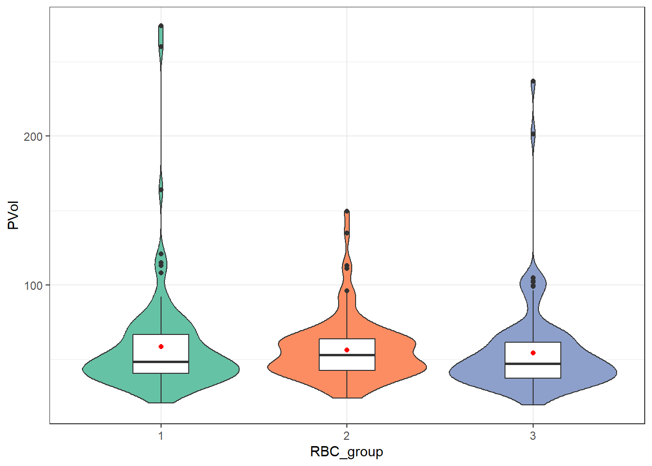

As when we’ve worked with other comparisons using independent samples, our main question is whether each sample appears likely to have come from a Normal distribution, or not. Here, all three RBC groups show meaningful (right) skew on the PVol outcome. We can see this with other tools as well, such as a set of faceted Normal Q-Q plots.

ggplot(storage, aes(sample = PVol, col = RBC_group)) +
  geom_qq() + geom_qq_line(aes(col = RBC_group)) +
  scale_color_metro_d() +
  facet_wrap(~ RBC_group, labeller = "label_both") +
  guides(color = "none") +
  labs(title = "Normal Q-Q plots of PVol by RBC_group",
       y = "Observed Data", x = "N(0,1) expectation")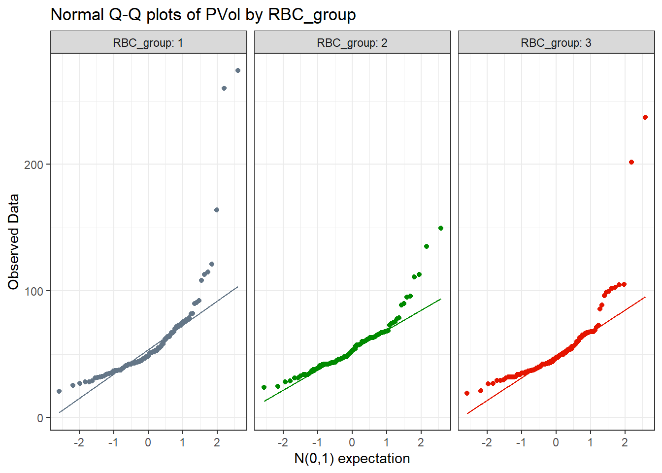

All three plots curve up and away from their respective straight lines at both the top and bottom of the distribution, indicating right skew.

Another approach we might use here comes from the ggdist package.

ggplot(storage, aes(y = RBC_group, x = PVol, fill = RBC_group)) +
  stat_slab(aes(thickness = after_stat(pdf * n)), scale = 0.7) +
  stat_dotsinterval(side = "bottom", scale = 0.7, slab_linewidth = NA) +
  scale_fill_brewer(palette = "Set2") +
  guides(fill = "none") +
  theme_bw()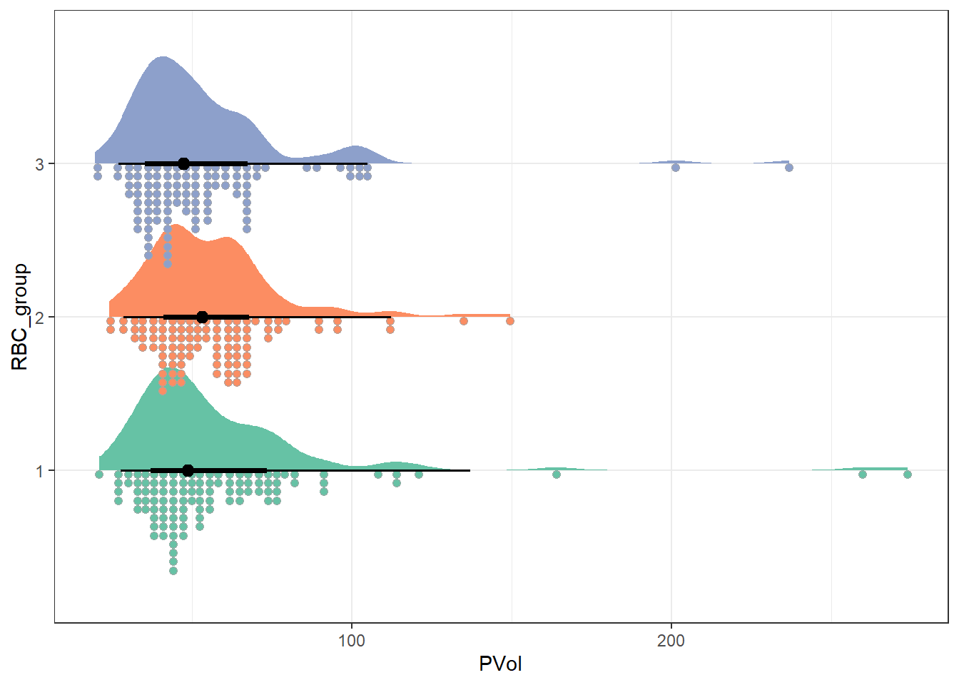

10.3.2 Numerical Summaries

Within each group, we see the mean PVol above the median PVol, also a sign of right skew.

storage |> 
  reframe(lovedist(PVol), .by = RBC_group) |>
  kable(digits = 2)

RBC_group	n	miss	mean	sd	med	mad	min	q25	q75	max
3	104	0	54.27	30.06	47.25	15.64	19.4	37.50	61.50	237.0
2	97	0	56.37	21.27	53.00	16.31	24.0	42.70	64.00	149.6
1	106	0	58.66	36.72	48.60	17.20	20.9	40.78	66.67	274.0

10.4 Initial Linear Fit

Despite the apparent right skew, let’s fit an OLS model (with lm()) first to the raw data, just for completeness.

fit1 <- lm(PVol ~ RBC_group, data = storage)

summary(fit1)

Call:
lm(formula = PVol ~ RBC_group, data = storage)

Residuals:
    Min      1Q  Median      3Q     Max 
-37.756 -16.174  -7.056   7.989 215.344 

Coefficients:
            Estimate Std. Error t value Pr(>|t|)    
(Intercept)   58.656      2.937  19.968   <2e-16 ***
RBC_group2    -2.289      4.249  -0.539    0.591    
RBC_group3    -4.382      4.174  -1.050    0.295    
---
Signif. codes:  0 '***' 0.001 '**' 0.01 '*' 0.05 '.' 0.1 ' ' 1

Residual standard error: 30.24 on 304 degrees of freedom
Multiple R-squared:  0.003615,  Adjusted R-squared:  -0.00294 
F-statistic: 0.5515 on 2 and 304 DF,  p-value: 0.5767

Under the fitted model, how would we interpret the point estimates?

• The intercept shows the average value of PVol for subjects in RBC_group1, the group not otherwise identfied here, and that is 58.7 grams.
• The RBC_group2 slope coefficient shows the average difference in PVol for subjects who were in RBC_group2 as compared to the baseline category: RBC_group1. That mean difference is estimated to be -2.3 grams, so that we estimate the mean PVol of RBC_group2 subjects to be 58.7 - 2.3 or 56.4 grams.
• Finally, the RBC_group3 slope coefficient shows the average difference in PVol for subjects who were in RBC_group3 as compared to RBC_group1. That mean difference is estimated to be -4.4 grams, so that we estimate the mean PVol of RBC_group3 subjects to be 58.7 - 4.4 or 54.3 grams.

Does the assumption of Normality required by this fit work well, according to the diagnostic Q-Q plot of residuals shown below?

plot(fit1, which = 2)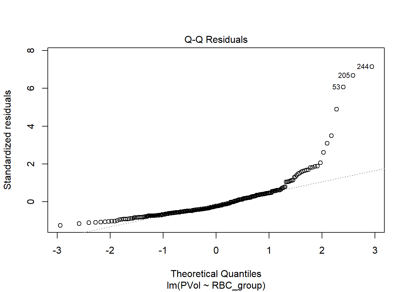

No. We still have lots of right skew, especially on the higher end of the residuals. Let’s consider transforming PVol.

10.5 Would a Transformation Be Useful?

boxCox(fit1, main = "Transformations of Prostate Volume")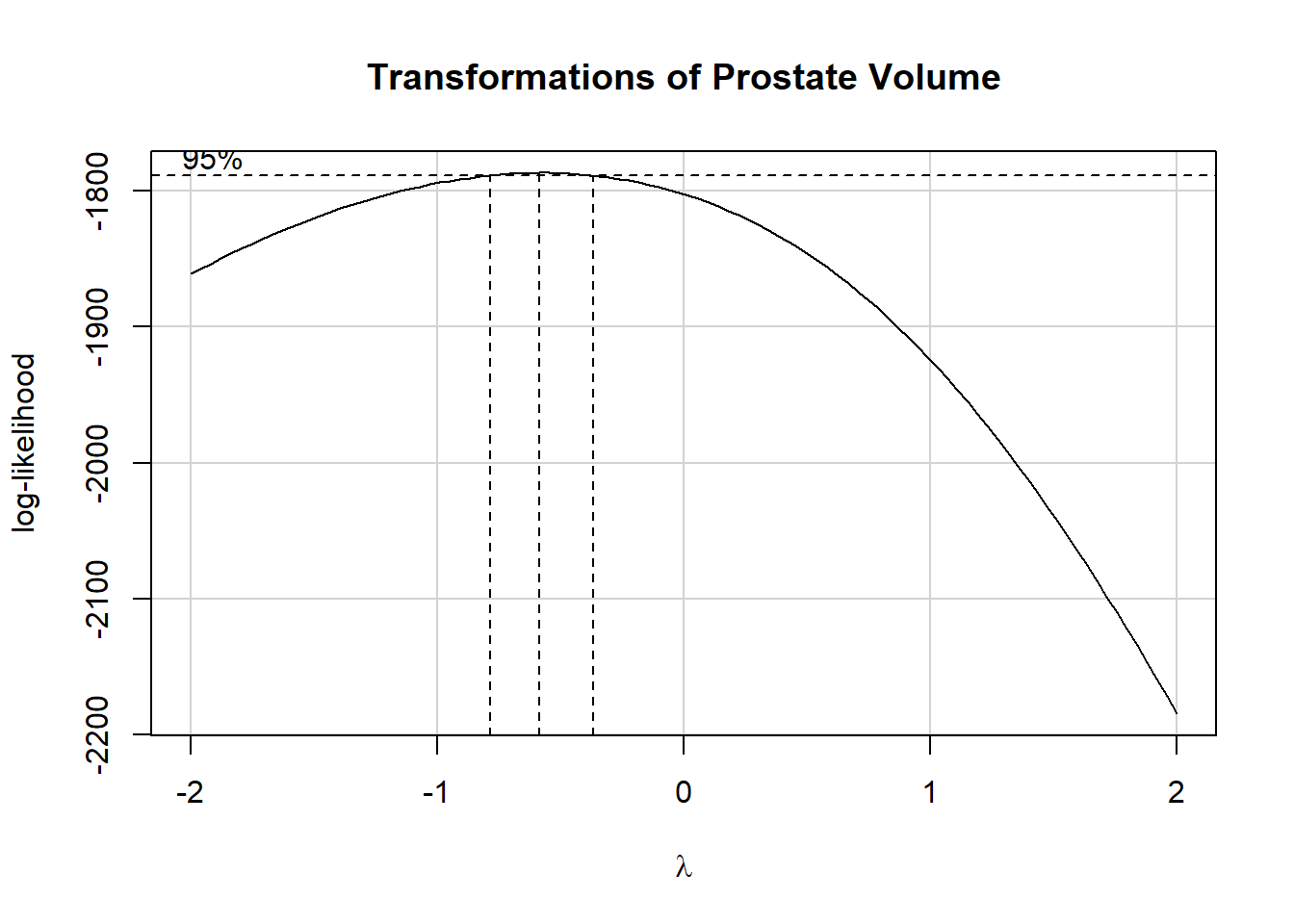

summary(powerTransform(fit1))$result

    Est Power Rounded Pwr Wald Lwr Bnd Wald Upr Bnd
Y1 -0.5717863        -0.5   -0.7825024   -0.3610701

Given the suggested power of -0.5, we’ll try an inverse square root, and compare it to the two nearest transformations, the log (power = 0) and the inverse (power = -1.) Here are a set of boxplots with means to help us.

p1 <- ggplot(storage, aes(x = log(PVol), y = RBC_group)) +
  geom_boxplot() +
  stat_summary(geom = "point", fun = "mean", size = 2, col = "red") +
  labs(title = "log(Prostate Volume)", y = "Group")

p2 <- ggplot(storage, aes(x = PVol^(-0.5), y = RBC_group)) +
  geom_boxplot() +
  stat_summary(geom = "point", fun = "mean", size = 2, col = "red") +
  labs(title = "Inverse Square Root of Prostate Volume", y = "Group")

p3 <- ggplot(storage, aes(x = 1/PVol, y = RBC_group)) +
  geom_boxplot() +
  stat_summary(geom = "point", fun = "mean", size = 2, col = "red") +
  labs(title = "1 / Prostate Volume", y = "Group")


p1 / p2 / p3 +
  plot_annotation(title = "Candidate Transformations")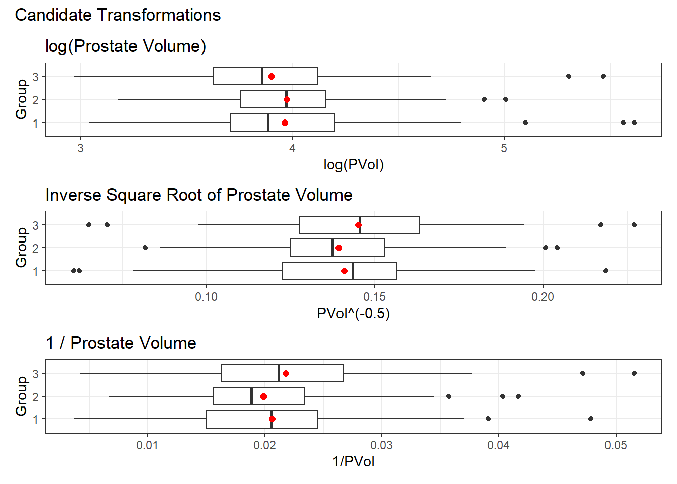

I think we could possibly go with any of these transformations, but I will select the inverse square root (power = -0.5) for two reasons:

• it has candidate outliers on both sides of the distribution, so it looks a little more symmetric than the other choices, and
• I haven’t used that transformation yet in this book.

10.5.1 Build in Transformation

Here are the means and standard deviations of the raw PVol values after our transformation.

storage |> group_by(RBC_group) |>
  summarise(mean = mean(PVol^(-0.5)), sd = sd(PVol^(-0.5)))

# A tibble: 3 × 3
  RBC_group  mean     sd
  <fct>     <dbl>  <dbl>
1 1         0.141 0.0274
2 2         0.139 0.0231
3 3         0.145 0.0272

I would want to multiply these values by a constant, say, 100, so that we can more easily look at the coefficients.

storage <- storage |> 
  mutate(PV_trans = 100*(PVol^(-0.5)))

storage |> group_by(RBC_group) |>
  summarise(mean = mean(PV_trans), sd = sd(PV_trans))

# A tibble: 3 × 3
  RBC_group  mean    sd
  <fct>     <dbl> <dbl>
1 1          14.1  2.74
2 2          13.9  2.31
3 3          14.5  2.72

10.6 Linear Fit after Inverse Square Root Transformation

fit2 <- lm(100*(PVol^(-0.5)) ~ RBC_group, data = storage)

summary(fit2)

Call:
lm(formula = 100 * (PVol^(-0.5)) ~ RBC_group, data = storage)

Residuals:
    Min      1Q  Median      3Q     Max 
-8.0487 -1.6050  0.0207  1.5161  8.1997 

Coefficients:
            Estimate Std. Error t value Pr(>|t|)    
(Intercept)  14.0899     0.2532  55.637   <2e-16 ***
RBC_group2   -0.1756     0.3664  -0.479    0.632    
RBC_group3    0.4142     0.3599   1.151    0.251    
---
Signif. codes:  0 '***' 0.001 '**' 0.01 '*' 0.05 '.' 0.1 ' ' 1

Residual standard error: 2.607 on 304 degrees of freedom
Multiple R-squared:  0.008931,  Adjusted R-squared:  0.002411 
F-statistic:  1.37 on 2 and 304 DF,  p-value: 0.2557

plot(fit2, which = 2)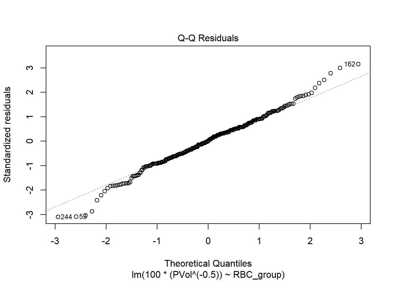

After this transformation, the Normal Q-Q plot of residuals is certainly closer to a Normal distribution. Is this also better than, say, the log transformation?

10.7 Linear Fit after Log Transformation

fit3 <- lm(log(PVol) ~ RBC_group, data = storage)

summary(fit3)

Call:
lm(formula = log(PVol) ~ RBC_group, data = storage)

Residuals:
     Min       1Q   Median       3Q      Max 
-0.93428 -0.23894 -0.04056  0.20666  1.65158 

Coefficients:
            Estimate Std. Error t value Pr(>|t|)    
(Intercept)  3.96155    0.03825 103.576   <2e-16 ***
RBC_group2   0.01084    0.05533   0.196    0.845    
RBC_group3  -0.06199    0.05435  -1.141    0.255    
---
Signif. codes:  0 '***' 0.001 '**' 0.01 '*' 0.05 '.' 0.1 ' ' 1

Residual standard error: 0.3938 on 304 degrees of freedom
Multiple R-squared:  0.006664,  Adjusted R-squared:  0.0001289 
F-statistic:  1.02 on 2 and 304 DF,  p-value: 0.3619

plot(fit3, which = 2)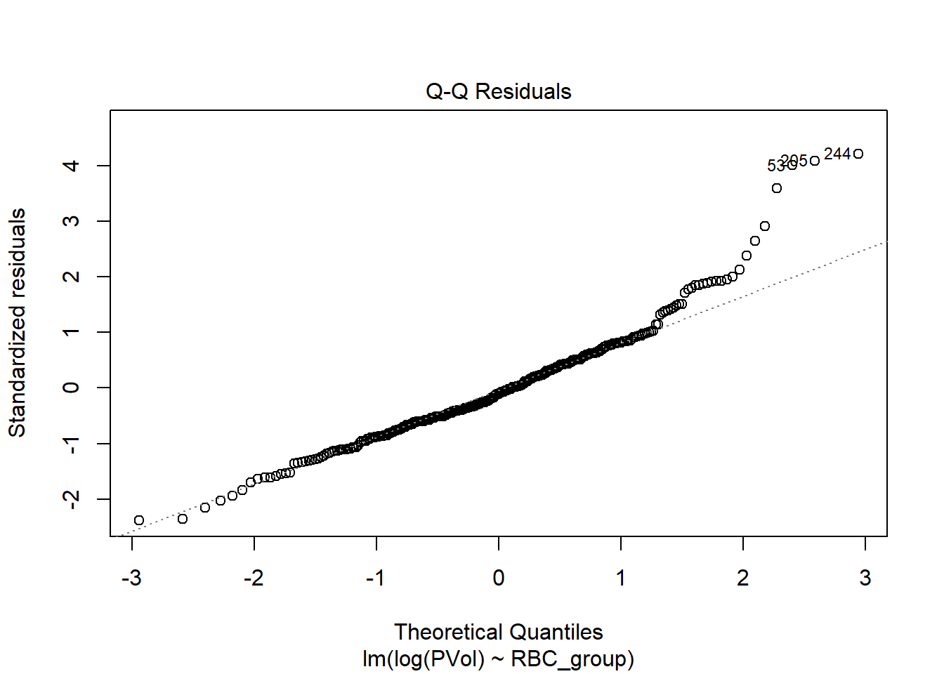

I think I prefer the inverse square root transformation here.

10.8 Back-Transforming Predictions

Let’s get that fit’s (fit2) predictions for each RBC_group:

estimate_means(fit2, ci = 0.95)

We selected `by = c("RBC_group")`.

Warning in (function (object, at, cov.reduce = mean, cov.keep = get_emm_option("cov.keep"), : There are unevaluated constants in the response formula
Auto-detection of the response transformation may be incorrect

Estimated Marginal Means

RBC_group | Mean |       SE |       95% CI
------------------------------------------
1         | 0.14 | 2.53e-03 | [0.14, 0.15]
2         | 0.14 | 2.65e-03 | [0.13, 0.14]
3         | 0.15 | 2.56e-03 | [0.14, 0.15]

Marginal means estimated at RBC_group

Note that we could also use:

estimate_expectation(fit2, data = "grid", ci = 0.95)

Model-based Expectation

RBC_group | Predicted |   SE |         95% CI
---------------------------------------------
1         |     14.09 | 0.25 | [13.59, 14.59]
2         |     13.91 | 0.26 | [13.39, 14.44]
3         |     14.50 | 0.26 | [14.00, 15.01]

Variable predicted: PVol
Predictors modulated: RBC_group

So, for example, our predicted transformed value of PVol among subjects in RBC_group 1 is 14.09, with 95% CI (13.59, 14.59).

To back-transform, we remember that the transformation we used was:

\[PVol_{transformed} = \frac{100}{\sqrt{PVol}}\]

To back out of the transformation we need to solve for PVol in terms of the transformed PVol. That is:

\[ PVol_{transformed} = \frac{100}{\sqrt{PVol}} \\ \frac{PVol_{transformed}}{100} = \frac{1}{\sqrt{PVol}} \\ \sqrt{PVol} = \frac{100}{PVol_{transformed}} \\ PVol = \left(\frac{100}{PVol_{transformed}}\right)^2 \]

Again, our predicted transformed value of PVol among subjects in RBC_group 1 is 14.09, with 95% CI (13.59, 14.59).

Converting these values back to our original scale (in g) for PVol gives:

• point estimate (100/14.09)^2 = 50.4
• lower bound (100/14.59)^2 = 47, and
• upper bound (100/13.59)^2 = 54.1

I’ll leave it to you to do the same sort of calculation for the point estimate and 95% CI for RBC groups 2 and 3.

10.9 Pairwise Comparisons of Means

10.9.1 Bonferroni correction approach

con1 <- estimate_contrasts(fit2, contrast = "RBC_group", 
                           ci = 0.95, p_adjust = "bonferroni")

Warning in (function (object, at, cov.reduce = mean, cov.keep = get_emm_option("cov.keep"), : There are unevaluated constants in the response formula
Auto-detection of the response transformation may be incorrect

con1 |> kable(digits = 2)

Level1	Level2	Difference	CI_low	CI_high	SE	df	t	p
RBC_group1	RBC_group2	0.18	-0.71	1.06	0.37	304	0.48	1.00
RBC_group1	RBC_group3	-0.41	-1.28	0.45	0.36	304	-1.15	0.75
RBC_group2	RBC_group3	-0.59	-1.48	0.30	0.37	304	-1.60	0.33

Note that each of these contrasts have confidence intervals which include zero. Is that still true with our other approaches?

10.9.2 Holm-Bonferroni approach

con2 <- estimate_contrasts(fit2, contrast = "RBC_group", 
                           ci = 0.95, p_adjust = "holm")

Warning in (function (object, at, cov.reduce = mean, cov.keep = get_emm_option("cov.keep"), : There are unevaluated constants in the response formula
Auto-detection of the response transformation may be incorrect

con2 |> kable(digits = 2)

Level1	Level2	Difference	CI_low	CI_high	SE	df	t	p
RBC_group1	RBC_group2	0.18	-0.71	1.06	0.37	304	0.48	0.63
RBC_group1	RBC_group3	-0.41	-1.28	0.45	0.36	304	-1.15	0.50
RBC_group2	RBC_group3	-0.59	-1.48	0.30	0.37	304	-1.60	0.33

10.9.3 Tukey HSD approach

con3 <- estimate_contrasts(fit2, contrast = "RBC_group", 
                           ci = 0.95, p_adjust = "tukey")

Warning in (function (object, at, cov.reduce = mean, cov.keep = get_emm_option("cov.keep"), : There are unevaluated constants in the response formula
Auto-detection of the response transformation may be incorrect

con3 |> kable(digits = 2)

Level1	Level2	Difference	CI_low	CI_high	SE	df	t	p
RBC_group1	RBC_group2	0.18	-0.69	1.04	0.37	304	0.48	0.88
RBC_group1	RBC_group3	-0.41	-1.26	0.43	0.36	304	-1.15	0.48
RBC_group2	RBC_group3	-0.59	-1.46	0.28	0.37	304	-1.60	0.25

10.10 Bayesian Linear Model

We can, of course, run a Bayesian linear model on our transformed outcome, too.

set.seed(431)
fit4 <- stan_glm(PV_trans ~ RBC_group, data = storage, refresh = 0)

post4 <- describe_posterior(fit4, ci = 0.95)

print_md(post4, digits = 2)

Summary of Posterior Distribution

Parameter	Median	95% CI	pd	ROPE	% in ROPE	Rhat	ESS
(Intercept)	14.09	[13.57, 14.61]	100%	[-0.26, 0.26]	0%	1.000	3480.00
RBC_group2	-0.17	[-0.91, 0.54]	68.40%	[-0.26, 0.26]	50.53%	1.000	3158.00
RBC_group3	0.41	[-0.32, 1.12]	86.10%	[-0.26, 0.26]	32.42%	1.000	3476.00

As before, we can obtain estimated predictions from this model with, for instance:

estimate_means(fit4, ci = 0.95)

We selected `by = c("RBC_group")`.

Estimated Marginal Means

RBC_group |  Mean |         95% CI |   pd
-----------------------------------------
1         | 14.09 | [13.57, 14.61] | 100%
2         | 13.92 | [13.40, 14.43] | 100%
3         | 14.51 | [14.00, 15.00] | 100%

Marginal means estimated at RBC_group

and again, we can back-transform these means and 95% credible intervals.

10.11 For More Information

1. Again, the Chapter on Inference for comparing many means in Çetinkaya-Rundel and Hardin (2024) is a good starting place for some people.
2. David Scott’s sections on Box-Cox transformations, Tukey Ladder of Powers and on Analysis of Variance: One-Factor may be helpful to you.
3. Andrea Onofri had some useful examples using the emmeans package in her 2019 tutorial Stabilising transformations: how do I present my results?

Cata, Juan P, Eric A. Klein, and Gerald A. Hoeltge et al. 2011. “Blood Storage Duration and Biochemical Recurrence of Cancer After Radical Prostatectomy.” Mayo Clinic Proceedings 86(2): 120–27. https://doi.org/10.4065/mcp.2010.0313.

Çetinkaya-Rundel, Mine, and Johanna Hardin. 2024. Introduction to Modern Statistics. Second Edition. OpenIntro Project. https://openintro-ims.netlify.app/.

Higgins, Peter. 2023. “Medicaldata: Data Package for Medical Datasets.” https://higgi13425.github.io/medicaldata/.

---

1. Note that the first author’s last name is Cata, not Cato, as the CCF repository suggests.