22 Multiple Regression and Imputation

This is a DRAFT version of this Chapter.

This is a sketchy draft. I’ll remove this notice when I post a version of this Chapter that is essentially finished.

22.1 R setup for this chapter

Note

Appendix A lists all R packages used in this book, and also provides R session information. Appendix B describes the 431-Love.R script, and demonstrates its use.

library(broom)
library(car)
library(ggmice)
library(glmnet)
library(janitor)
library(knitr)
library(mice)
library(naniar)
library(olsrr)
library(patchwork)
library(rstanarm)

library(easystats)
library(tidyverse)

source("data/Love-431.R")
theme_set(theme_bw())

22.2 Data will be Countries of the World version 2

Note

Appendix C provides further guidance on pulling data from other systems into R, while Appendix D gives more information (including download links) for all data sets used in this book.

ctry <- read_csv("data/countries.csv", show_col_types = FALSE) |>
  mutate(
    UNIV_CARE = factor(UNIV_CARE),
    WHO_REGION = factor(WHO_REGION),
    WBANK_INCOME = factor(WBANK_INCOME),
    C_NUM = as.character(C_NUM)
  ) |>
  janitor::clean_names()

ctry

# A tibble: 192 × 14
   c_num country_name    hale_all univ_care wbank_income hale_2000 births_attend
   <chr> <chr>              <dbl> <fct>     <fct>            <dbl>         <dbl>
 1 1     Afghanistan         50.4 no        Low               46.8            68
 2 2     Albania             66.7 yes       Upper-middle      65.2           100
 3 3     Algeria             65.5 yes       Lower-middle      62.7            99
 4 4     Andorra             NA   no        High              NA             100
 5 5     Angola              53.8 no        Lower-middle      42.9            50
 6 6     Antigua and Ba…     66.5 no        High              65.5            99
 7 7     Argentina           64.8 yes       Upper-middle      65.1            99
 8 8     Armenia             64   no        Upper-middle      63.5           100
 9 9     Australia           70.6 yes       High              68.6            99
10 10    Austria             69.8 yes       High              68.2            98
# ℹ 182 more rows
# ℹ 7 more variables: ihr_core_cap <dbl>, avg_tempc <dbl>, female_22 <dbl>,
#   rural_22 <dbl>, covid_vax100 <dbl>, who_region <fct>, iso_alpha3 <chr>

miss_var_summary(ctry)

# A tibble: 14 × 3
   variable      n_miss pct_miss
   <chr>          <int>    <num>
 1 births_attend     20   10.4  
 2 hale_all           9    4.69 
 3 hale_2000          9    4.69 
 4 covid_vax100       6    3.12 
 5 ihr_core_cap       2    1.04 
 6 wbank_income       1    0.521
 7 c_num              0    0    
 8 country_name       0    0    
 9 univ_care          0    0    
10 avg_tempc          0    0    
11 female_22          0    0    
12 rural_22           0    0    
13 who_region         0    0    
14 iso_alpha3         0    0

miss_case_table(ctry)

# A tibble: 4 × 3
  n_miss_in_case n_cases pct_cases
           <int>   <int>     <dbl>
1              0     164     85.4 
2              1      16      8.33
3              2       5      2.60
4              3       7      3.65

Outcome HALE_ALL
3 categorical variables (UNIV_CARE, WHO_REGION, WBANK_INCOME)
8 quantitative predictors (HALE_2000, BIRTHS_ATTEND, IHR_CORE_CAP, AVG_TEMPC, FEMALE_22, RURAL_22, COVID_VAX100)

and some missing values (at least in the predictors) to deal with…

22.3 Build single imputation

22.3.1 Filter out countries without information on our outcome, `hale_all`.

ctry_cc <- ctry |>
  filter(complete.cases(hale_all))

pct_miss_case(ctry_cc)

[1] 10.38251

Later, when we do multiple imputation, we’ll run 15 imputations.

22.3.2 Single Imputation

ctry_si <- 
  mice(ctry_cc, m = 1, seed = 431, print = FALSE) |>
  complete() |>
  tibble()

Warning: Number of logged events: 3

dim(ctry_si)

[1] 183  14

n_miss(ctry_si)

[1] 0

22.3.3 Partition data after single imputation

We’ve seen other ways to partition the data. Here, let’s use data_partition() from the datawizard package, part of the easystats ecosystem.

out <- data_partition(ctry_si, proportion = 0.7, seed = 431)

ctry_si_train <- out$p_0.7
ctry_si_test <- out$test

dim(ctry_si_train)

[1] 128  15

dim(ctry_si_test)

[1] 55 15

22.4 Transforming the outcome?

fit0 <- lm(
  hale_all ~ univ_care + wbank_income +
    hale_2000 + births_attend + ihr_core_cap +
    avg_tempc + female_22 + rural_22 + covid_vax100,
  data = ctry_si_train
)

boxCox(fit0)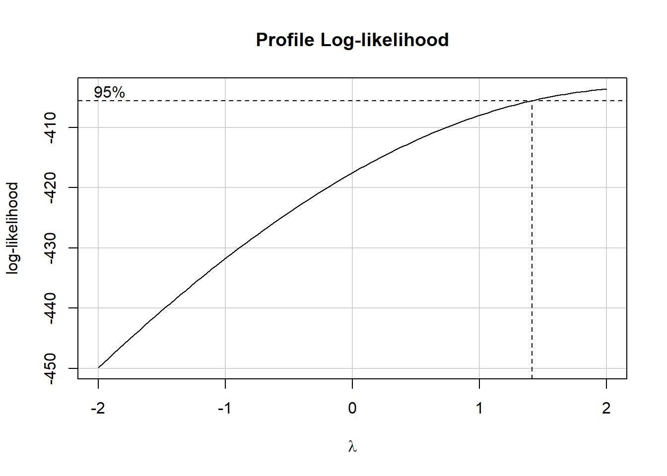

Let’s try the square of hale_all as our outcome.

p1 <- ggplot(ctry_si_train, aes(x = hale_all)) +
  geom_histogram(bins = 20, fill = "coral", col = "blue")

p2 <- ggplot(ctry_si_train, aes(x = hale_all^2)) +
  geom_histogram(bins = 20, fill = "aquamarine", col = "blue")

p1 + p2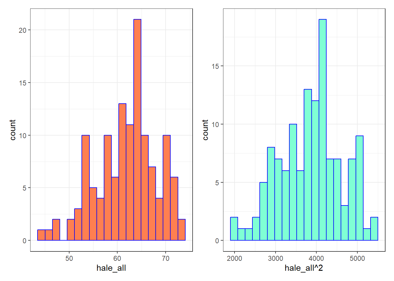

Not much of a difference, but perhaps we will see more meaningful improvements in our regression residual plots.

ctry_si_train <- ctry_si_train |>
  mutate(hale_sqr = hale_all^2)

ctry_si_test <- ctry_si_test |>
  mutate(hale_sqr = hale_all^2)

22.5 Fitting and Evaluating in Training Data

22.5.1 Kitchen Sink Model

fit1 <- lm( hale_sqr ~ 
              univ_care + wbank_income + hale_2000 + births_attend +
              ihr_core_cap + avg_tempc + female_22 + rural_22 + 
              covid_vax100,
  data = ctry_si_train
)

model_parameters(fit1)

Parameter                   | Coefficient |     SE |              95% CI | t(116) |      p
------------------------------------------------------------------------------------------
(Intercept)                 |     -291.03 | 598.75 | [-1476.93,  894.86] |  -0.49 | 0.628 
univ care [yes]             |       44.22 |  61.01 | [  -76.62,  165.05] |   0.72 | 0.470 
wbank income [Low]          |      -28.88 | 140.59 | [ -307.33,  249.58] |  -0.21 | 0.838 
wbank income [Lower-middle] |     -186.50 |  98.98 | [ -382.54,    9.54] |  -1.88 | 0.062 
wbank income [Upper-middle] |     -284.94 |  74.59 | [ -432.67, -137.21] |  -3.82 | < .001
hale 2000                   |       59.94 |   5.05 | [   49.94,   69.94] |  11.87 | < .001
births attend               |        4.81 |   2.11 | [    0.64,    8.99] |   2.28 | 0.024 
ihr core cap                |        4.65 |   1.87 | [    0.96,    8.35] |   2.49 | 0.014 
avg tempc                   |       -5.48 |   3.75 | [  -12.91,    1.95] |  -1.46 | 0.147 
female 22                   |       -2.05 |   9.07 | [  -20.01,   15.91] |  -0.23 | 0.822 
rural 22                    |        1.67 |   1.62 | [   -1.54,    4.89] |   1.03 | 0.305 
covid vax100                |        3.02 |   1.28 | [    0.49,    5.56] |   2.36 | 0.020


Uncertainty intervals (equal-tailed) and p-values (two-tailed) computed
  using a Wald t-distribution approximation.

model_performance(fit1)

# Indices of model performance

AIC      |     AICc |      BIC |    R2 | R2 (adj.) |    RMSE |   Sigma
----------------------------------------------------------------------
1807.365 | 1810.558 | 1844.441 | 0.888 |     0.878 | 254.555 | 267.398

22.5.2 LASSO to identify a subset

pred_x <- model.matrix(fit1)
out_y <- ctry_si_train |> select(hale_sqr) |> as.matrix()

set.seed(431)
lasso <- cv.glmnet(x = pred_x, y = out_y,
                   type.measure = "mse",
                   alpha = 1, family = "gaussian",
                   nlambda = 200, nfolds = 10)

plot(lasso)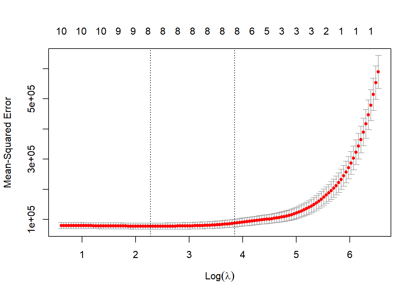

log(lasso$lambda.min)

[1] 2.275831

predict(lasso, type = "coef", s = "lambda.min")

13 x 1 sparse Matrix of class "dgCMatrix"
                          lambda.min
(Intercept)              -222.093827
(Intercept)                 .       
univ_careyes               29.607576
wbank_incomeLow             .       
wbank_incomeLower-middle -129.930275
wbank_incomeUpper-middle -241.669217
hale_2000                  58.555358
births_attend               4.299195
ihr_core_cap                4.520508
avg_tempc                  -4.936356
female_22                   .       
rural_22                    .       
covid_vax100                2.959860

The LASSO suggestion is to drop two of the 9 variables in our original fit1 model, specifcally female_22 and rural_22, since wbank_income is multi-categorical.

So that model would be:

fit7 <- lm( hale_sqr ~ 
              univ_care + wbank_income + hale_2000 + births_attend +
              ihr_core_cap + avg_tempc + covid_vax100,
  data = ctry_si_train
)

22.5.3 Stepwise Approach

fit6 <- select_parameters(fit1)

compare_models(fit1, fit6)

Parameter                   |                        fit1 |                       fit6
--------------------------------------------------------------------------------------
(Intercept)                 | -291.03 (-1476.93,  894.86) | -288.36 (-992.56,  415.84)
wbank income (Low)          |  -28.88 ( -307.33,  249.58) |    1.23 (-263.48,  265.94)
wbank income (Lower-middle) | -186.50 ( -382.54,    9.54) | -165.91 (-343.22,   11.40)
wbank income (Upper-middle) | -284.94 ( -432.67, -137.21) | -280.72 (-421.53, -139.91)
hale 2000                   |   59.94 (   49.94,   69.94) |   59.16 (  49.52,   68.80)
births attend               |    4.81 (    0.64,    8.99) |    4.96 (   0.83,    9.10)
ihr core cap                |    4.65 (    0.96,    8.35) |    4.58 (   1.08,    8.09)
avg tempc                   |   -5.48 (  -12.91,    1.95) |   -5.42 ( -11.86,    1.01)
covid vax100                |    3.02 (    0.49,    5.56) |    3.08 (   0.61,    5.55)
univ care (yes)             |   44.22 (  -76.62,  165.05) |                           
rural 22                    |    1.67 (   -1.54,    4.89) |                           
female 22                   |   -2.05 (  -20.01,   15.91) |                           
--------------------------------------------------------------------------------------
Observations                |                         128 |                        128

The stepwise approach drops three predictors, univ_care, rural_22 and female_22.

22.5.4 Best Subsets

How about using the best subsets approach?

k <- ols_step_best_subset(fit1, 
                          max_order = 7,
                          metric = "cp")

                                    Best Subsets Regression                                     
------------------------------------------------------------------------------------------------
Model Index    Predictors
------------------------------------------------------------------------------------------------
     1         hale_2000                                                                         
     2         wbank_income hale_2000                                                            
     3         wbank_income hale_2000 ihr_core_cap                                               
     4         wbank_income hale_2000 births_attend ihr_core_cap                                 
     5         wbank_income hale_2000 births_attend ihr_core_cap covid_vax100                    
     6         wbank_income hale_2000 births_attend ihr_core_cap avg_tempc covid_vax100          
     7         wbank_income hale_2000 births_attend ihr_core_cap avg_tempc rural_22 covid_vax100 
------------------------------------------------------------------------------------------------

                                                           Subsets Regression Summary                                                            
-------------------------------------------------------------------------------------------------------------------------------------------------
                       Adj.        Pred                                                                                                           
Model    R-Square    R-Square    R-Square     C(p)         AIC         SBIC          SBC           MSEP             FPE          HSP        APC  
-------------------------------------------------------------------------------------------------------------------------------------------------
  1        0.8151      0.8136      0.8073    68.3017    1852.0658    1487.2564    1860.6218    13968177.2014    110831.2677    873.0094    0.1908 
  2        0.8556      0.8509       0.842    32.1908    1826.4294    1458.2510    1843.5416    10997356.3890     89354.3939    704.0977    0.1514 
  3        0.8724      0.8672      0.8573    16.6786    1812.5604    1445.0276    1832.5246     9794054.7936     80190.2350    632.1970    0.1358 
  4        0.8794      0.8734      0.8632    11.4137    1807.3525    1440.3096    1830.1687     9333656.2974     77004.7739    607.4578    0.1304 
  5        0.8844      0.8777      0.8668     8.1680    1803.8834    1437.4087    1829.5516     9017164.5402     74958.1159    591.7503    0.1269 
  6        0.8871      0.8795      0.8675     7.4172    1802.9193    1436.9166    1831.4396     8884176.1798     74408.9130    587.9223    0.1260 
  7        0.8879      0.8794      0.8666     8.5288    1803.9471    1438.2545    1835.3194     8891046.5054     75023.3563    593.3632    0.1270 
-------------------------------------------------------------------------------------------------------------------------------------------------
AIC: Akaike Information Criteria 
 SBIC: Sawa's Bayesian Information Criteria 
 SBC: Schwarz Bayesian Criteria 
 MSEP: Estimated error of prediction, assuming multivariate normality 
 FPE: Final Prediction Error 
 HSP: Hocking's Sp 
 APC: Amemiya Prediction Criteria

plot(k)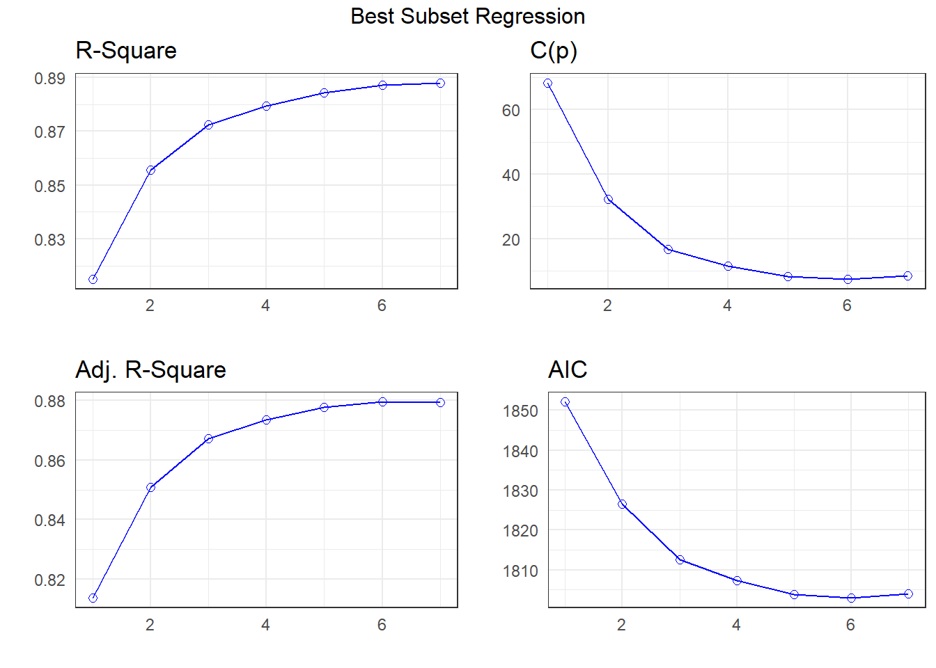

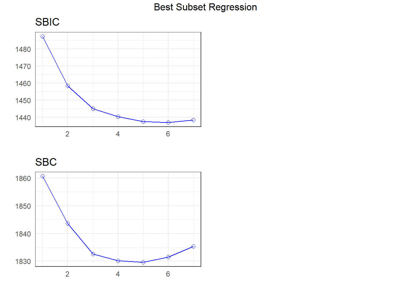
The best subsets suggestions include

the same six-predictor model we got with stepwise
a five-predictor model with avg_tempc dropped from our 6-predictor model, and maybe
a different seven-parameter model than we obtained from the LASSO (keeping rural_22 but dropping univ_care)

Let’s store the five-predictor model:

fit5 <- lm( hale_sqr ~ 
              wbank_income + hale_2000 + births_attend +
              ihr_core_cap + covid_vax100,
  data = ctry_si_train
)

22.5.5 Compare Candidate Models in Training Sample

So we have at least four candidate models: fit1, fit5, fit6 and fit7.

compare_models(fit1, fit7, fit6, fit5)

Parameter                   |                        fit1 |                       fit7 |                       fit6 |                        fit5
-------------------------------------------------------------------------------------------------------------------------------------------------
(Intercept)                 | -291.03 (-1476.93,  894.86) | -263.05 (-974.18,  448.09) | -288.36 (-992.56,  415.84) | -439.16 (-1125.27,  246.94)
wbank income (Low)          |  -28.88 ( -307.33,  249.58) |    1.60 (-263.85,  267.06) |    1.23 (-263.48,  265.94) |  -33.50 ( -296.90,  229.91)
wbank income (Lower-middle) | -186.50 ( -382.54,    9.54) | -157.94 (-337.70,   21.81) | -165.91 (-343.22,   11.40) | -194.85 ( -370.09,  -19.62)
wbank income (Upper-middle) | -284.94 ( -432.67, -137.21) | -279.75 (-420.99, -138.52) | -280.72 (-421.53, -139.91) | -300.61 ( -440.45, -160.78)
hale 2000                   |   59.94 (   49.94,   69.94) |   58.86 (  49.13,   68.58) |   59.16 (  49.52,   68.80) |   59.49 (   49.78,   69.19)
births attend               |    4.81 (    0.64,    8.99) |    4.87 (   0.71,    9.02) |    4.96 (   0.83,    9.10) |    5.29 (    1.15,    9.44)
ihr core cap                |    4.65 (    0.96,    8.35) |    4.42 (   0.87,    7.98) |    4.58 (   1.08,    8.09) |    5.04 (    1.55,    8.53)
covid vax100                |    3.02 (    0.49,    5.56) |    3.00 (   0.50,    5.49) |    3.08 (   0.61,    5.55) |    2.86 (    0.39,    5.34)
univ care (yes)             |   44.22 (  -76.62,  165.05) |   35.15 ( -81.32,  151.62) |                            |                            
female 22                   |   -2.05 (  -20.01,   15.91) |                            |                            |                            
avg tempc                   |   -5.48 (  -12.91,    1.95) |   -5.35 ( -11.81,    1.10) |   -5.42 ( -11.86,    1.01) |                            
rural 22                    |    1.67 (   -1.54,    4.89) |                            |                            |                            
-------------------------------------------------------------------------------------------------------------------------------------------------
Observations                |                         128 |                        128 |                        128 |                         128

compare_performance(fit1, fit7, fit6, fit5)

# Comparison of Model Performance Indices

Name | Model |  AIC (weights) | AICc (weights) |  BIC (weights) |    R2 | R2 (adj.) |    RMSE |   Sigma
-------------------------------------------------------------------------------------------------------
fit1 |    lm | 1807.4 (0.050) | 1810.6 (0.026) | 1844.4 (<.001) | 0.888 |     0.878 | 254.555 | 267.398
fit7 |    lm | 1804.5 (0.206) | 1806.8 (0.170) | 1835.9 (0.029) | 0.887 |     0.879 | 255.719 | 266.334
fit6 |    lm | 1802.9 (0.460) | 1804.8 (0.463) | 1831.4 (0.272) | 0.887 |     0.879 | 256.106 | 265.614
fit5 |    lm | 1803.9 (0.284) | 1805.4 (0.341) | 1829.6 (0.699) | 0.884 |     0.878 | 259.088 | 267.585

plot(compare_performance(fit1, fit7, fit6, fit5))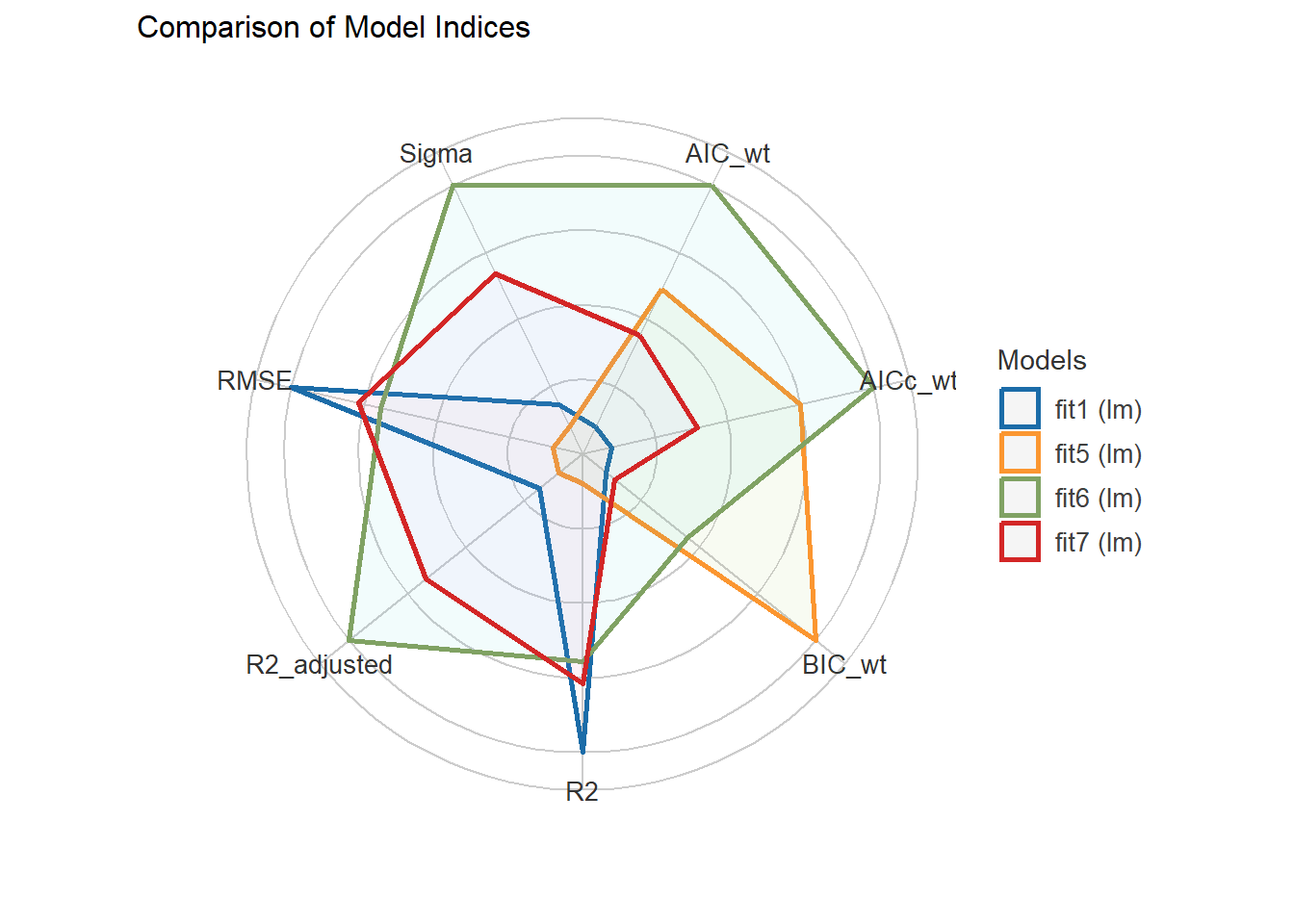

It looks like the six-predictor model is the best choice (but just barely) using adjusted \(R^2\), \(\sigma\) and AIC. Let’s look at the test sample.

22.5.6 Compare Candidate Models in Test Sample

test1 <- augment(fit1, newdata = ctry_si_test) |>
  mutate(mod_n = "Model 1 (KS)")
test7 <- augment(fit7, newdata = ctry_si_test) |>
  mutate(mod_n = "Model 7")
test6 <- augment(fit6, newdata = ctry_si_test) |>
  mutate(mod_n = "Model 6")
test5 <- augment(fit5, newdata = ctry_si_test) |>
  mutate(mod_n = "Model 5")

test_res <- bind_rows(test1, test7, test6, test5) |>
  mutate(predicted_haleall = sqrt(.fitted),
         resid_haleall = hale_all - predicted_haleall) |>
  select(mod_n, country_name, hale_all, 
         predicted_haleall, resid_haleall, everything()) |>
  arrange(c_num, mod_n)

head(test_res, 8)

# A tibble: 8 × 21
  mod_n    country_name hale_all predicted_haleall resid_haleall c_num univ_care
  <chr>    <chr>           <dbl>             <dbl>         <dbl> <chr> <fct>    
1 Model 1… Luxembourg       71.2              68.6          2.55 100   yes      
2 Model 5  Luxembourg       71.2              68.5          2.68 100   yes      
3 Model 6  Luxembourg       71.2              68.7          2.49 100   yes      
4 Model 7  Luxembourg       71.2              68.8          2.39 100   yes      
5 Model 1… Maldives         66.7              63.8          2.90 104   yes      
6 Model 5  Maldives         66.7              63.6          3.15 104   yes      
7 Model 6  Maldives         66.7              63.2          3.53 104   yes      
8 Model 7  Maldives         66.7              63.3          3.38 104   yes      
# ℹ 14 more variables: wbank_income <fct>, hale_2000 <dbl>,
#   births_attend <dbl>, ihr_core_cap <dbl>, avg_tempc <dbl>, female_22 <dbl>,
#   rural_22 <dbl>, covid_vax100 <dbl>, who_region <fct>, iso_alpha3 <chr>,
#   .row_id <int>, hale_sqr <dbl>, .fitted <dbl>, .resid <dbl>

test_res |> 
    group_by(mod_n) |>
    summarise(MAPE = mean(abs(resid_haleall)),
              medAPE = median(abs(resid_haleall)),
              maxAPE = max(abs(resid_haleall)),
              RMSPE = sqrt(mean(resid_haleall^2)),
              rsqr = cor(hale_all, predicted_haleall)^2) |>
  kable()

mod_n	MAPE	medAPE	maxAPE	RMSPE	rsqr
Model 1 (KS)	1.399561	1.172160	4.242786	1.682548	0.9063445
Model 5	1.387650	1.091875	3.818286	1.700453	0.9009602
Model 6	1.357642	1.198238	4.019098	1.660509	0.9072666
Model 7	1.347411	1.168969	3.973297	1.637438	0.9092709

We see that:

Model 6 has the smallest mean, median and maximum average prediction error, but
Model 7 has the smallest RMSPE and largest validated \(R^2\).

I’ll select model 6, assuming that model assumptions aren’t too badly violated in our training sample. Let’s check that.

22.6 Check Assumptions in Winning Model

check_model(fit6)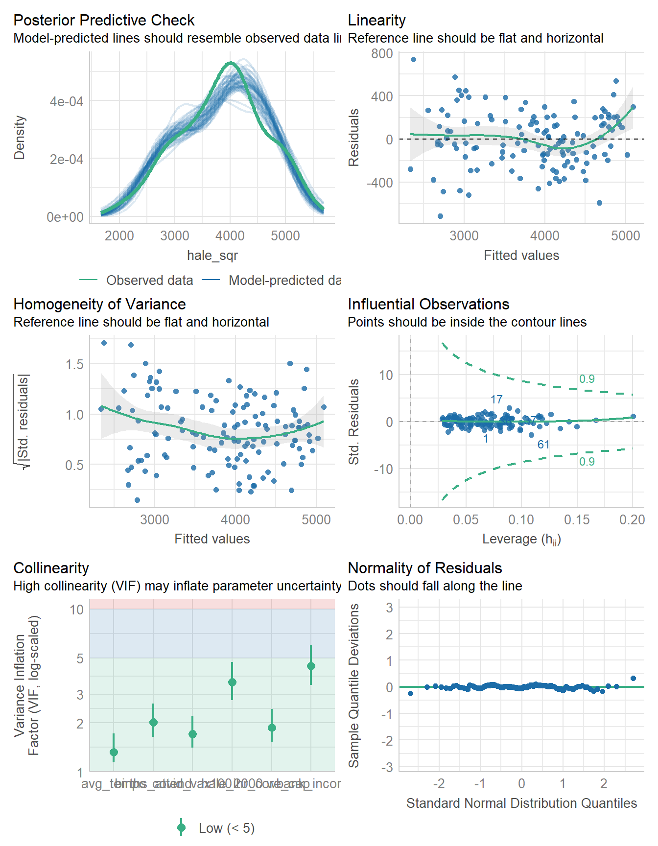

The collinearity is OK now, and outside of a couple of observations, I think Normality isn’t a serious problem.

22.7 Estimates for the Winning Model

So now, I’ll refit the six-predictor model, which includes:

wbank_income
hale_2000
births_attend
ihr_core_cap
avg_tempc, and
covid_vax100

to the entire set of data, with various assumptions about the missing data.

22.7.1 Complete Case Analysis

Here, we’ll fit the model to all of the data except (as we’ll do in all three cases) the countries without outcome (hale_all) information.

fit_cc <- lm((hale_all^2) ~ wbank_income + hale_2000 +
               births_attend + ihr_core_cap +
               avg_tempc + covid_vax100,
             data = ctry_cc)

model_parameters(fit_cc, ci = 0.95)

Parameter                   | Coefficient |     SE |             95% CI | t(155) |      p
-----------------------------------------------------------------------------------------
(Intercept)                 |      -93.51 | 302.42 | [-690.90,  503.89] |  -0.31 | 0.758 
wbank income [Low]          |      -68.39 | 112.63 | [-290.88,  154.11] |  -0.61 | 0.545 
wbank income [Lower-middle] |     -148.19 |  73.52 | [-293.42,   -2.97] |  -2.02 | 0.046 
wbank income [Upper-middle] |     -267.91 |  60.30 | [-387.02, -148.81] |  -4.44 | < .001
hale 2000                   |       57.44 |   4.20 | [  49.14,   65.74] |  13.67 | < .001
births attend               |        4.84 |   1.79 | [   1.31,    8.37] |   2.71 | 0.008 
ihr core cap                |        3.80 |   1.51 | [   0.81,    6.79] |   2.51 | 0.013 
avg tempc                   |       -5.51 |   2.80 | [ -11.05,    0.03] |  -1.97 | 0.051 
covid vax100                |        2.65 |   1.09 | [   0.49,    4.81] |   2.42 | 0.017


Uncertainty intervals (equal-tailed) and p-values (two-tailed) computed
  using a Wald t-distribution approximation.

model_performance(fit_cc)

# Indices of model performance

AIC       |      AICc |       BIC |    R2 | R2 (adj.) |    RMSE |   Sigma
-------------------------------------------------------------------------
44110.965 | 44112.403 | 44141.963 | 0.881 |     0.874 | 247.017 | 254.088

22.7.2 After Single Imputation

fit_si <- lm((hale_all^2) ~ wbank_income + hale_2000 +
               births_attend + ihr_core_cap +
               avg_tempc + covid_vax100,
             data = ctry_si)

model_parameters(fit_si, ci = 0.95)

Parameter                   | Coefficient |     SE |             95% CI | t(174) |      p
-----------------------------------------------------------------------------------------
(Intercept)                 |      -49.82 | 270.59 | [-583.88,  484.25] |  -0.18 | 0.854 
wbank income [Low]          |      -79.91 |  97.08 | [-271.51,  111.69] |  -0.82 | 0.412 
wbank income [Lower-middle] |     -178.92 |  65.89 | [-308.97,  -48.86] |  -2.72 | 0.007 
wbank income [Upper-middle] |     -293.54 |  56.08 | [-404.22, -182.87] |  -5.23 | < .001
hale 2000                   |       57.96 |   3.67 | [  50.72,   65.20] |  15.80 | < .001
births attend               |        4.50 |   1.63 | [   1.29,    7.72] |   2.76 | 0.006 
ihr core cap                |        3.75 |   1.41 | [   0.97,    6.53] |   2.66 | 0.008 
avg tempc                   |       -6.47 |   2.60 | [ -11.60,   -1.35] |  -2.49 | 0.014 
covid vax100                |        2.64 |   0.98 | [   0.70,    4.57] |   2.69 | 0.008


Uncertainty intervals (equal-tailed) and p-values (two-tailed) computed
  using a Wald t-distribution approximation.

model_performance(fit_si)

# Indices of model performance

AIC       |      AICc |       BIC |    R2 | R2 (adj.) |    RMSE |   Sigma
-------------------------------------------------------------------------
52919.799 | 52921.078 | 52951.894 | 0.892 |     0.887 | 239.530 | 245.647

22.7.3 Multiple Imputation

As mentioned earlier, I am dropping the observations with no information on my outcome (hale_all) which is the ctry_cc data. Then I am building 15 imputations, because I am missing data on just over 10% of cases within ctry_cc.

pct_miss_case(ctry_cc) # as a reminder

[1] 10.38251

Now, we fit our six-predictor model in each of these 15 imputed data sets, like this:

imp_ests <- ctry_cc |>
  mice(m = 15, seed = 431, print = FALSE) |>
  with(lm((hale_all)^2 ~ wbank_income + hale_2000 +
               births_attend + ihr_core_cap +
               avg_tempc + covid_vax100)) |>
  pool()

Warning: Number of logged events: 3

model_parameters(imp_ests, ci = 0.95)

Warning: Number of logged events: 3
Warning: Number of logged events: 3
Warning: Number of logged events: 3
Warning: Number of logged events: 3

# Fixed Effects

Parameter                   | Coefficient |     SE |             95% CI |     t |     df |      p
-------------------------------------------------------------------------------------------------
(Intercept)                 |      -66.57 | 274.03 | [-607.55,  474.42] | -0.24 | 168.60 | 0.808 
wbank income [Low]          |      -74.63 |  97.66 | [-267.42,  118.15] | -0.76 | 169.38 | 0.446 
wbank income [Lower-middle] |     -172.29 |  66.57 | [-303.70,  -40.88] | -2.59 | 170.49 | 0.010 
wbank income [Upper-middle] |     -294.49 |  56.44 | [-405.89, -183.09] | -5.22 | 171.96 | < .001
hale 2000                   |       58.20 |   3.69 | [  50.91,   65.49] | 15.76 | 169.20 | < .001
births attend               |        4.50 |   1.66 | [   1.23,    7.77] |  2.72 | 166.98 | 0.007 
ihr core cap                |        3.70 |   1.42 | [   0.91,    6.50] |  2.62 | 171.40 | 0.010 
avg tempc                   |       -6.47 |   2.61 | [ -11.62,   -1.32] | -2.48 | 171.81 | 0.014 
covid vax100                |        2.70 |   1.01 | [   0.72,    4.68] |  2.69 | 171.28 | 0.008


Uncertainty intervals (equal-tailed) and p-values (two-tailed) computed
  using a Wald t-distribution approximation.

glance(imp_ests)

  nimp nobs r.squared adj.r.squared
1   15  183 0.8915267     0.8865394

and hopefully show them all to be fairly similar. Then describe that winning fit in some detail, probably in the multiple imputation case.

22.8 Bayesian Linear Fit

Show Bayesian fit for the winning model across the entire sample, and draw conclusions about its fit and form.

ctry_si <- ctry_si |>
  mutate(hale_sqr = hale_all^2)

fit_bay <- stan_glm(hale_sqr ~ 
                      wbank_income + hale_2000 +
                      births_attend + ihr_core_cap +
                      avg_tempc + covid_vax100,
                    data = ctry_si, refresh = 0)

model_parameters(fit_bay, ci = 0.95)

Parameter                |  Median |             95% CI |     pd |  Rhat |     ESS |                       Prior
----------------------------------------------------------------------------------------------------------------
(Intercept)              |  -58.22 | [-593.32,  491.26] | 58.45% | 1.000 | 2586.00 | Normal (3859.71 +- 1825.71)
wbank_incomeLow          |  -79.75 | [-272.32,  116.58] | 78.38% | 1.001 | 2311.00 |    Normal (0.00 +- 5057.64)
wbank_incomeLower-middle | -177.89 | [-309.74,  -47.08] | 99.50% | 1.000 | 2335.00 |    Normal (0.00 +- 4014.05)
wbank_incomeUpper-middle | -292.57 | [-409.28, -179.50] |   100% | 1.001 | 3126.00 |    Normal (0.00 +- 4111.90)
hale_2000                |   58.05 | [  50.54,   64.89] |   100% | 1.001 | 3029.00 |     Normal (0.00 +- 209.73)
births_attend            |    4.54 | [   1.29,    7.67] | 99.72% | 1.000 | 4459.00 |     Normal (0.00 +- 113.08)
ihr_core_cap             |    3.74 | [   0.99,    6.54] | 99.55% | 1.000 | 4377.00 |     Normal (0.00 +- 101.06)
avg_tempc                |   -6.43 | [ -11.52,   -1.41] | 99.33% | 1.000 | 4533.00 |     Normal (0.00 +- 225.51)
covid_vax100             |    2.60 | [   0.68,    4.50] | 99.62% | 1.000 | 4575.00 |      Normal (0.00 +- 74.26)


Uncertainty intervals (equal-tailed) and p-values (two-tailed) computed
  using a MCMC distribution approximation.

model_performance(fit_bay)

# Indices of model performance

ELPD      | ELPD_SE |    LOOIC | LOOIC_SE |     WAIC |    R2 | R2 (adj.) |    RMSE |   Sigma
--------------------------------------------------------------------------------------------
-1272.992 |  10.426 | 2545.984 |   20.853 | 2545.895 | 0.887 |     0.880 | 239.536 | 246.897

22.9 For More Information

point to https://r4ds.hadley.nz/missing-values

22.1 R setup for this chapter

22.2 Data will be Countries of the World version 2

22.3 Build single imputation

22.3.1 Filter out countries without information on our outcome, hale_all.

22.3.2 Single Imputation

22.3.3 Partition data after single imputation

22.4 Transforming the outcome?

22.5 Fitting and Evaluating in Training Data

22.5.1 Kitchen Sink Model

22.5.2 LASSO to identify a subset

22.5.3 Stepwise Approach

22.5.4 Best Subsets

22.5.5 Compare Candidate Models in Training Sample

22.5.6 Compare Candidate Models in Test Sample

22.6 Check Assumptions in Winning Model

22.7 Estimates for the Winning Model

22.7.1 Complete Case Analysis

22.7.2 After Single Imputation

22.7.3 Multiple Imputation

22.8 Bayesian Linear Fit

22.9 For More Information

22.3.1 Filter out countries without information on our outcome, `hale_all`.