12  Studying Craters

12.1 R setup for this chapter

Note

Appendix A lists all R packages used in this book, and also provides R session information. Appendix B describes the 431-Love.R script, and demonstrates its use.

library(glue)
library(haven)
library(janitor)
library(knitr)
library(naniar)
library(patchwork)
library(rstanarm)

library(easystats)
library(tidyverse)

source("data/Love-431.R")
theme_set(theme_bw())

12.2 Data from an SPSS File: Craters

Note

Appendix C provides further guidance on pulling data from other systems into R, while Appendix D gives more information (including download links) for all data sets used in this book.

These data are adapted from the Data and Story Library, which provides the following introduction to the data which were originally gathered from the Earth Impact Database:

Meteor Crater in Arizona was the first recognized impact crater and was identified as such only in the 1920s. With the help of satellite images, more and more craters have been identified; now more than 180 are known. These, of course, are only a small sample of all the impacts the earth has experienced: Only 29% of earth’s surface is land, and many craters have been covered or eroded away. Astronomers have recog-nized a roughly 35 million-year cycle in the frequency of cratering, although the cause of this cycle is not fully understood.

The data hold information about craters. craters from the most recent 35Ma (million years) may be the more reliable data, and are suitable for analyses relating age and diameter.

Craters are large indentations in the ground, usually bowl-shaped, and caused by the impact of some sort of celestial object. Our data come from an SPSS format (.sav) and can be ingested into R using the read_sav() function from the haven package.

craters <- read_sav("data/craters.sav") |>
  janitor::clean_names()

craters

# A tibble: 168 × 10
   crater name          diameter     age n_s   latitude longitude buried drilled
    <dbl> <chr>            <dbl>   <dbl> <dbl>    <dbl>     <dbl> <dbl+> <dbl+l>
 1      1 "Haviland"       0.015 1   e-3 1 [N]     37.6     -99.2 1 [N]  1 [N]  
 2      2 "Dalgaranga"     0.024 2.7 e-1 2 [S]    -27.6     117.  1 [N]  1 [N]  
 3      3 "Sikhote Ali…    0.027 5.50e-5 1 [N]     46.1     135.  1 [N]  1 [N]  
 4      4 "Campo Del C…    0.05  4   e-3 2 [S]    -27.6     -61.7 1 [N]  2 [Y]  
 5      5 "Sobolev"        0.053 1   e-3 1 [N]     46.3     138.  1 [N]  2 [Y]  
 6      6 "Veevers"        0.08  1   e+0 2 [S]    -23.0     125.  1 [N]  1 [N]  
 7      7 "Ilumets\u00…    0.08  2   e-3 1 [N]     58.0      27.4 1 [N]  2 [Y]  
 8      8 "Morasko"        0.1   1   e-2 1 [N]     52.5      16.9 1 [N]  1 [N]  
 9      9 "Kaalij\u008…    0.11  4   e-3 1 [N]     58.4      22.7 1 [N]  1 [N]  
10     10 "Wabar"          0.116 1.4 e-4 1 [N]     21.5      50.5 1 [N]  1 [N]  
# ℹ 158 more rows
# ℹ 1 more variable: location <chr>

Columns in the data include:

Variable	Description
crater	numerical code (1 - 168)
name	name of crater
diameter	diameter in km
age	age in millions of years (mA)
n_s	(N)orthern or (S)outhern hemisphere
latitude	Latitude, in degrees N or S of the equator
longitude	Longitude, in degrees W or E of the Greenwich meridian
buried	Yes or No
drilled	Yes or No
location	country (and sometimes state or province)

craters |> count(drilled)

# A tibble: 3 × 2
  drilled       n
  <dbl+lbl> <int>
1  1 [N]       67
2  2 [Y]       96
3 NA            5

str(craters)

tibble [168 × 10] (S3: tbl_df/tbl/data.frame)
 $ crater   : num [1:168] 1 2 3 4 5 6 7 8 9 10 ...
  ..- attr(*, "format.spss")= chr "F8.2"
 $ name     : chr [1:168] "Haviland" "Dalgaranga" "Sikhote Alin" "Campo Del Cielo" ...
  ..- attr(*, "format.spss")= chr "A42"
 $ diameter : num [1:168] 0.015 0.024 0.027 0.05 0.053 0.08 0.08 0.1 0.11 0.116 ...
  ..- attr(*, "format.spss")= chr "F8.2"
 $ age      : num [1:168] 1.0e-03 2.7e-01 5.5e-05 4.0e-03 1.0e-03 1.0 2.0e-03 1.0e-02 4.0e-03 1.4e-04 ...
  ..- attr(*, "format.spss")= chr "F8.2"
 $ n_s      : dbl+lbl [1:168] 1, 2, 1, 2, 1, 2, 1, 1, 1, 1, 2, 1, 2, 1, 1, 1, 2, 2, ...
   ..@ format.spss: chr "F8.0"
   ..@ labels     : Named num [1:2] 1 2
   .. ..- attr(*, "names")= chr [1:2] "N" "S"
 $ latitude : num [1:168] 37.6 -27.6 46.1 -27.6 46.3 ...
  ..- attr(*, "format.spss")= chr "F8.2"
 $ longitude: num [1:168] -99.2 117.3 134.7 -61.7 137.9 ...
  ..- attr(*, "format.spss")= chr "F8.2"
 $ buried   : dbl+lbl [1:168] 1, 1, 1, 1, 1, 1, 1, 1, 1, 1, 1, 1, 1, 1, 1, 1, 1, 1, ...
   ..@ format.spss: chr "F8.0"
   ..@ labels     : Named num [1:2] 1 2
   .. ..- attr(*, "names")= chr [1:2] "N" "Y"
 $ drilled  : dbl+lbl [1:168]  1,  1,  1,  2,  2,  1,  2,  1,  1,  1,  1,  2,  1,  1...
   ..@ format.spss: chr "F8.0"
   ..@ labels     : Named num [1:2] 1 2
   .. ..- attr(*, "names")= chr [1:2] "N" "Y"
 $ location : chr [1:168] "Kansas, U.S.A." "Western Australia, Australia" "Russia" "Argentina" ...
  ..- attr(*, "format.spss")= chr "A36"

As we can see, several of the columns are labeled, and we likely want to eliminate those labels in our R code. To do so, we can use zap_labels() from the haven package.

craters <- craters |> zap_labels() |>
  mutate(buried = fct_recode(factor(buried), "No" = "1", "Yes" = "2"),
         drilled = fct_recode(factor(drilled), "No" = "1", "Yes" = "2"))

summary(craters)

     crater           name              diameter            age           
 Min.   :  1.00   Length:168         Min.   :  0.015   Min.   :   0.0001  
 1st Qu.: 42.75   Class :character   1st Qu.:  3.150   1st Qu.:  36.9000  
 Median : 84.50   Mode  :character   Median :  8.000   Median : 124.5000  
 Mean   : 84.50                      Mean   : 18.713   Mean   : 266.2618  
 3rd Qu.:126.25                      3rd Qu.: 18.250   3rd Qu.: 383.7500  
 Max.   :168.00                      Max.   :300.000   Max.   :2400.0000  
      n_s           latitude        longitude         buried    drilled  
 Min.   :1.000   Min.   :-34.72   Min.   :-156.633   No  :105   No  :67  
 1st Qu.:1.000   1st Qu.: 22.56   1st Qu.: -80.858   Yes : 61   Yes :96  
 Median :1.000   Median : 46.98   Median :  18.333   NA's:  2   NA's: 5  
 Mean   :1.208   Mean   : 33.94   Mean   :   2.892                       
 3rd Qu.:1.000   3rd Qu.: 56.68   3rd Qu.:  48.642                       
 Max.   :2.000   Max.   : 75.70   Max.   : 172.083                       
   location        
 Length:168        
 Class :character  
 Mode  :character  
                   
                   
                   

12.3 Association of age and diameter

res1 <- craters |> reframe(lovedist(age)) |> mutate(varname = "age")
res2 <- craters |> reframe(lovedist(diameter)) |> mutate(varname = "diameter")

rbind(res1, res2) |> relocate(varname) |> kable(digits = 2)

varname	n	miss	mean	sd	med	mad	min	q25	q75	max
age	168	0	266.26	379.03	124.5	183.69	0.00	36.90	383.75	2400
diameter	168	0	18.71	36.37	8.0	8.27	0.01	3.15	18.25	300

The age and diameter data each appear to be right skewed, with the sample mean substantially larger than the sample median, and the points clustered more closely together at the left of the histograms.

p1 <- ggplot(craters, aes(x = age)) +
  geom_histogram(bins = 12, fill = "salmon", col = "beige") +
  labs(title = "Age in millions of years (mA)")

p2 <- ggplot(craters, aes(x = diameter)) +
  geom_histogram(bins = 12, fill = "forestgreen", col = "beige") +
  labs(title = "Diameter in km")

(p1 + p2) + 
  plot_annotation(title = "Age and Diameter of Craters",
                  subtitle = "Histograms, n = 168 craters")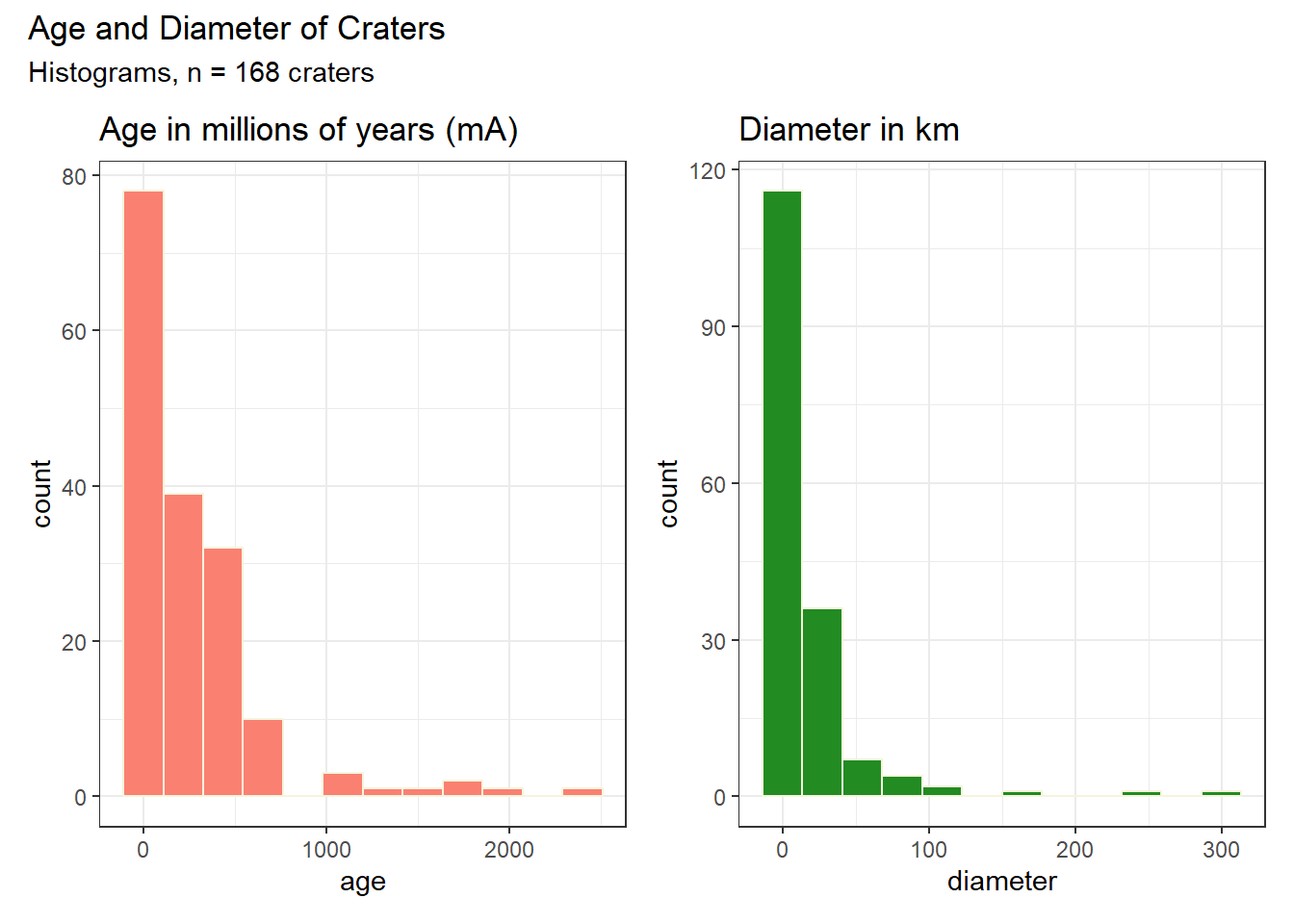

When we look at the scatterplot of the association between age and diameter, most of the points are gathered in the bottom left of the plot.

ggplot(craters, aes(x = age, y = diameter)) +
  geom_point() +
  geom_smooth(method = "lm", formula = y ~ x, col = "red") + 
  annotate("text", x = 500, y = 250, 
           label = glue("Pearson r = ", 
                        round(cor(craters$age, craters$diameter),2)))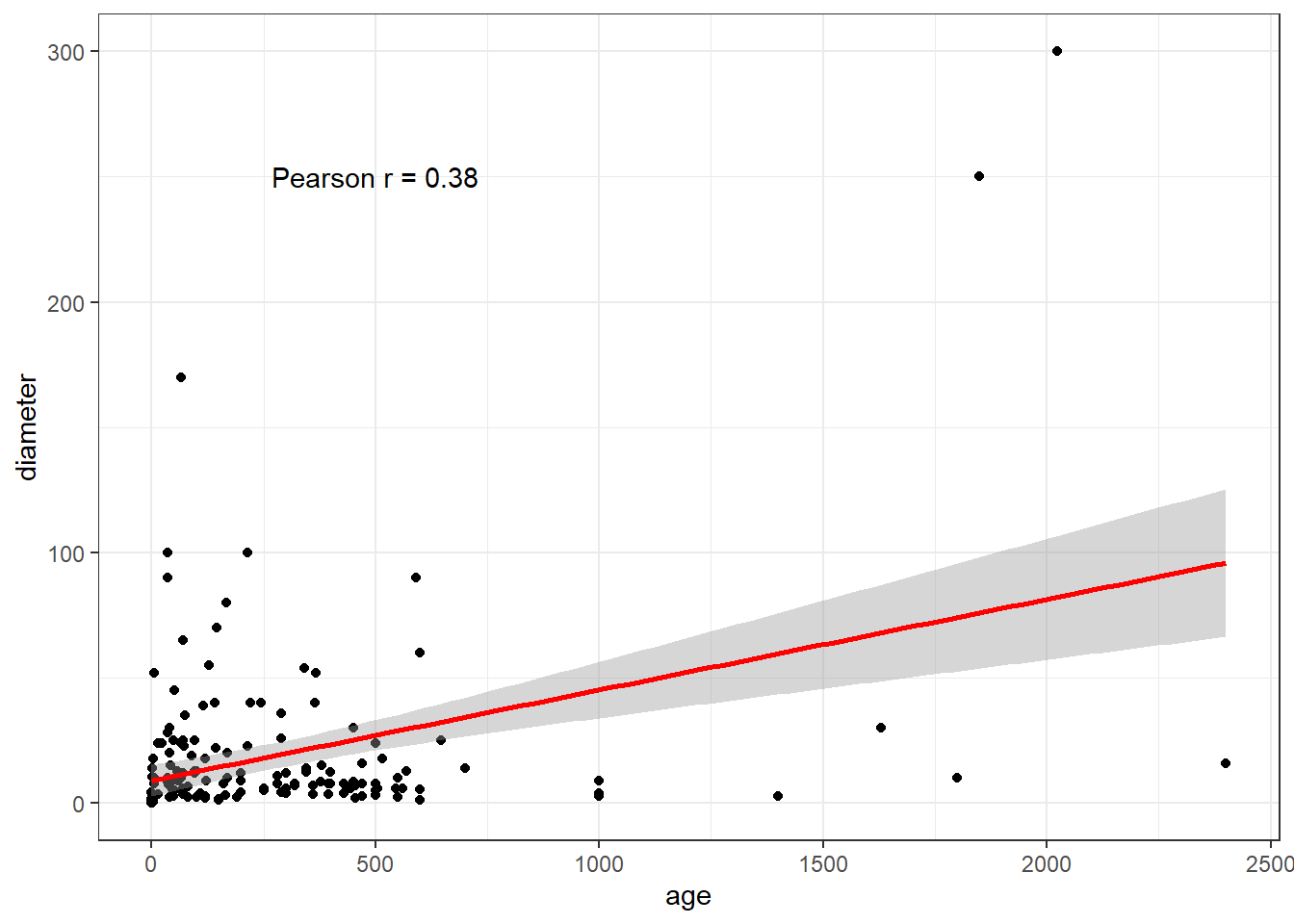

In light of these results, it may be that a transformation (of either age, diameter or both) is in order.

12.4 Logarithmic Transformation of Each Variable

Consider taking the logarithm of both age and diameter.

What does this imply? From Gelman, Hill, and Vehtari (2021) Section 3.4:

• The formula log y = a + b log x describes what is called power-law growth (if b > 0) or decline (if b < 0), with the formula \(y = Ax^b\) where A = exp(a).
• The parameter A is the value of y when x = 1
• The parameter b determines the rate of growth or decline.
• A one-unit difference in log x corresponds to an additive difference of b in log y.
• One example is a power law: Let y be the area of a square and x be its perimeter. Then \(y = (x/4)^2\) and we can take the log of both sides to get log y = 2 (log x - log 4) = -2.8 + 2 log x.

12.4.1 Distributions after Transformation

We’d expect applying a log transformation to spread out the lower values, reducing the right skew in each variable. Is this what happens?

p3 <- ggplot(craters, aes(x = log(age))) +
  geom_histogram(bins = 12, fill = "salmon", col = "beige") +
  labs(title = "log(Age in millions of years)")

p4 <- ggplot(craters, aes(x = log(diameter))) +
  geom_histogram(bins = 12, fill = "forestgreen", col = "beige") +
  labs(title = "log(Diameter in km)")

(p3 + p4) + 
  plot_annotation(title = "Logarithms of Age and Diameter",
                  subtitle = "Histograms, n = 168 craters")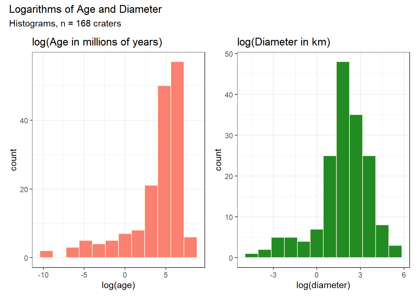

craters <- craters |>
  mutate(logage = log(age), logdiameter = log(diameter))

res3 <- craters |> reframe(lovedist(logage)) |> mutate(varname = "logage")
res4 <- craters |> reframe(lovedist(logdiameter)) |> mutate(varname = "logdiameter")

rbind(res3, res4) |> relocate(varname) |> kable(digits = 2)

varname	n	miss	mean	sd	med	mad	min	q25	q75	max
logage	168	0	3.76	3.46	4.82	1.71	-9.81	3.61	5.95	7.78
logdiameter	168	0	1.83	1.79	2.08	1.36	-4.20	1.15	2.90	5.70

Note that the means and medians after the logarithmic transformation are substantially closer to each other, as is indicated by the reduction in skew we see in the histograms.

12.4.2 Association after Transformation

What happens when we look at the scatterplot of these transformed variables?

ggplot(craters, aes(x = logage, y = logdiameter)) +
  geom_point() +
  geom_smooth(method = "lm", formula = y ~ x, col = "red") +
  annotate("text", x = -5, y = 5, 
           label = glue("Pearson r = ", 
                        round(cor(craters$logage, craters$logdiameter),2)))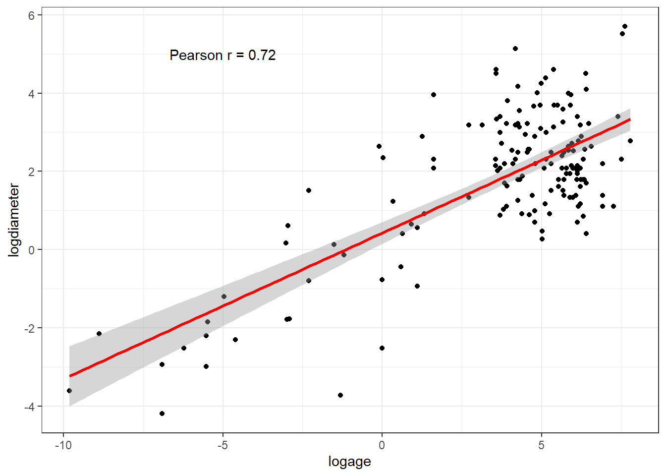

While we now have many points clustered in the top right of the plot, the overall fit of a linear model appears much better, as the points more closely cluster around the fitted line.

12.4.3 Comparing the Correlation Coefficients

We also see a larger Pearson correlation after this transformation, as we can also see from the cor_test() results below.

cor_test(craters, "age", "diameter")

Parameter1 | Parameter2 |    r |       95% CI | t(166) |         p
------------------------------------------------------------------
age        |   diameter | 0.38 | [0.24, 0.50] |   5.25 | < .001***

Observations: 168

cor_test(craters, "logage", "logdiameter")

Parameter1 |  Parameter2 |    r |       95% CI | t(166) |         p
-------------------------------------------------------------------
logage     | logdiameter | 0.72 | [0.64, 0.79] |  13.49 | < .001***

Observations: 168

We might also consider looking at the Spearman rank correlations:

cor_test(craters, "age", "diameter", method = "Spearman")

Parameter1 | Parameter2 |  rho |       95% CI |        S |         p
--------------------------------------------------------------------
age        |   diameter | 0.33 | [0.19, 0.46] | 5.28e+05 | < .001***

Observations: 168

cor_test(craters, "logage", "logdiameter", method = "Spearman")

Parameter1 |  Parameter2 |  rho |       95% CI |        S |         p
---------------------------------------------------------------------
logage     | logdiameter | 0.33 | [0.19, 0.46] | 5.28e+05 | < .001***

Observations: 168

Notice that the logarithmic transformation preserves the order of the observations, so that the ranks by age and diameter are identical to the ranks by log(age) and log(diameter), so the transformation has no impact on the Spearman rank correlation.

12.5 Untransformed Linear Model

fit1 <- lm(age ~ diameter, data = craters)

model_parameters(fit1, ci = 0.95) |> kable(digits = 2)

Parameter	Coefficient	SE	CI	CI_low	CI_high	t	df_error	p
(Intercept)	192.71	30.57	0.95	132.35	253.06	6.30	166	0
diameter	3.93	0.75	0.95	2.45	5.41	5.25	166	0

model_performance(fit1)

# Indices of model performance

AIC      |     AICc |      BIC |    R2 | R2 (adj.) |    RMSE |   Sigma
----------------------------------------------------------------------
2451.026 | 2451.172 | 2460.398 | 0.142 |     0.137 | 349.997 | 352.099

check_model(fit1)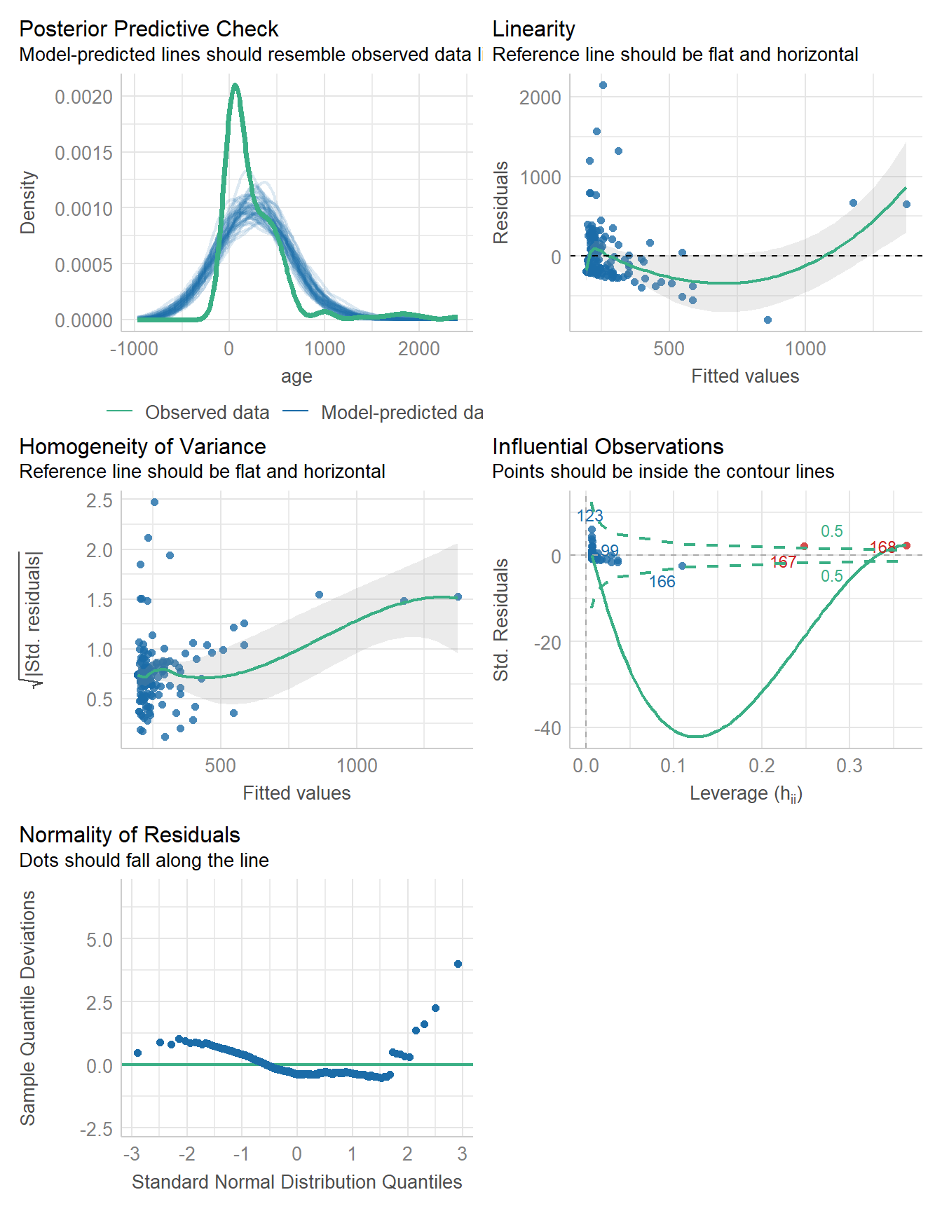

12.6 Log-Log Regression Model

fit3 <- lm(logage ~ logdiameter, data = craters)

model_parameters(fit3, ci = 0.95) |> kable(digits = 3)

Parameter	Coefficient	SE	CI	CI_low	CI_high	t	df_error	p
(Intercept)	1.199	0.265	0.95	0.675	1.723	4.52	166	0
logdiameter	1.401	0.104	0.95	1.196	1.606	13.49	166	0

model_performance(fit3)

# Indices of model performance

AIC     |    AICc |     BIC |    R2 | R2 (adj.) |  RMSE | Sigma
---------------------------------------------------------------
774.932 | 775.078 | 784.304 | 0.523 |     0.520 | 2.386 | 2.400

Our equation is log(age) = 1.2 + 1.4 log(diameter).

We can exponentiate both sides to see the relation between age and diameter on the untransformed scales.

\[ \exp(\log y) = \exp(1.2 + 1.4 \log(diameter)), \mbox{so } \\ y = exp(1.2) \times x^{1.4}, \mbox{so } y = 3.32 x^{1.4} \]

When increasing diameter by a factor of 2 (i.e., doubling the diameter) the estimated age is multiplied by \(2^{1.4} = 2.64\). Halving the diameter causes the estimated age to be multiplied by \((1/2)^{1.4} = 0.38\), and so forth.

check_model(fit3)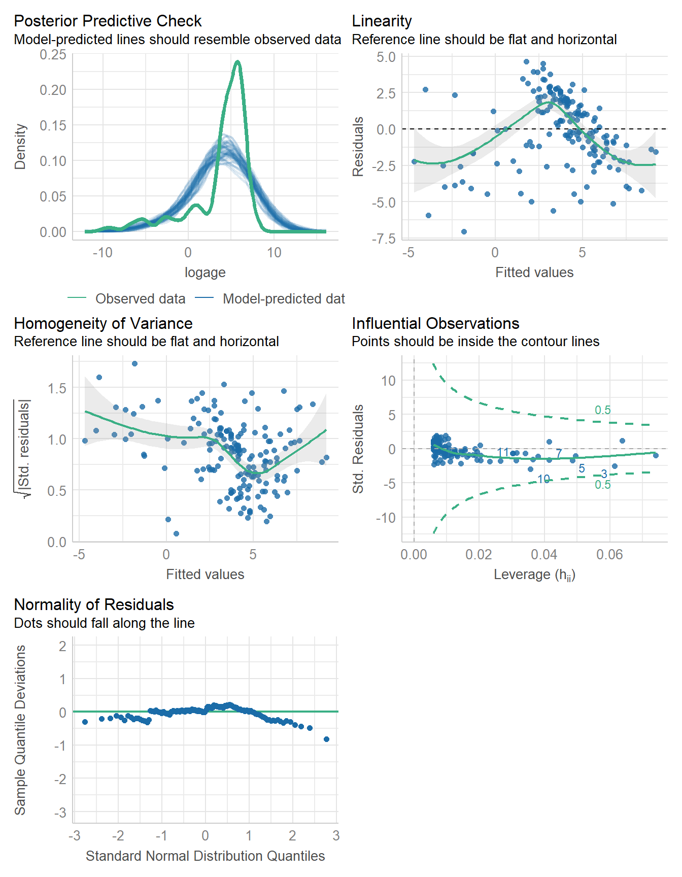

The fit is better here, although still not really as good as we might hope for. Would a Bayesian fit be helpful?

12.7 Bayesian Log-Log Regression

set.seed(431)
fit4 <- stan_glm(logage ~ logdiameter, 
                 data = craters, refresh = 0)

model_parameters(fit4, ci = 0.95) |> kable(digits = 2)

Parameter	Median	CI	CI_low	CI_high	pd	Rhat	ESS	Prior_Distribution	Prior_Location	Prior_Scale
(Intercept)	1.21	0.95	0.67	1.72	1	1	3756.99	normal	3.76	8.66
logdiameter	1.40	0.95	1.20	1.61	1	1	3860.42	normal	0.00	4.84

model_performance(fit4)

# Indices of model performance

ELPD     | ELPD_SE |   LOOIC | LOOIC_SE |    WAIC |    R2 | R2 (adj.) |  RMSE | Sigma
-------------------------------------------------------------------------------------
-387.860 |   8.599 | 775.720 |   17.198 | 775.699 | 0.519 |     0.508 | 2.386 | 2.411

check_model(fit4)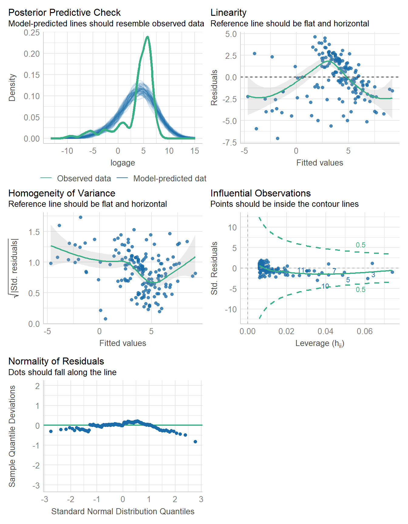

We still have some meaningful non-linearity, I think, but we’ll leave it as is for now.

12.8 For More Information

1. Gelman, Hill, and Vehtari (2021) is a great, though not free, reference for many of the ideas discussed in this entire book, and especially this chapter.
2. More on check_model() in Visual check of model assumptions. Posterior predictive checks is another good resource.
3. Chapter 7 of Çetinkaya-Rundel and Hardin (2024) is about linear regression with a single predictor, and has sections on residuals and checking for outliers, for instance.
4. The Qualtrics support page has a walkthrough for residual plots in the case of simple linear regression that should provide some additional background.

Çetinkaya-Rundel, Mine, and Johanna Hardin. 2024. Introduction to Modern Statistics. Second Edition. OpenIntro Project. https://openintro-ims.netlify.app/.

Gelman, Andrew, Jennifer Hill, and Aki Vehtari. 2021. Regression and Other Stories. New York: Cambridge University Press. https://avehtari.github.io/ROS-Examples/.