20  Multiple Regression with many predictors

This is a DRAFT version of this Chapter.

This is a sketchy draft. I’ll remove this notice when I post a version of this Chapter that is essentially finished.

20.1 R setup for this chapter

Note

Appendix A lists all R packages used in this book, and also provides R session information.

library(car)
library(janitor)
library(knitr)
library(naniar)
library(olsrr)
library(rstanarm)

library(easystats)
library(tidyverse)

theme_set(theme_bw())

Multiple regression y predicted by 3-15 variables

20.2 Data is bodyfat

Note

Appendix C provides further guidance on pulling data from other systems into R, while Appendix D gives more information (including download links) for all data sets used in this book.

My source for these data was Kaggle, although the data have been published in several other places. The data describe 252 men whose percentage of body fat was determined via underwater weighing and Siri’s (1956) equation.

From Kaggle:

These data are used to produce the predictive equations for lean body weight given in the abstract “Generalized body composition prediction equation for men using simple measurement techniques”, K.W. Penrose, A.G. Nelson, A.G. Fisher, FACSM, Human Performance Research Center, Brigham Young University, Provo, Utah 84602 as listed in Medicine and Science in Sports and Exercise, vol. 17, no. 2, April 1985, p. 189.

bodyfat <- read_csv("data/bodyfat.csv", show_col_types = FALSE) |>
  janitor::clean_names()

bodyfat

# A tibble: 248 × 16
   kag_row density siri_bf   age weight height  neck chest abdomen   hip thigh
   <chr>     <dbl>   <dbl> <dbl>  <dbl>  <dbl> <dbl> <dbl>   <dbl> <dbl> <dbl>
 1 sub_001    1.07    12.3    23   154.   67.8  36.2  93.1    85.2  94.5  59  
 2 sub_002    1.09     6.1    22   173.   72.2  38.5  93.6    83    98.7  58.7
 3 sub_003    1.04    25.3    22   154    66.2  34    95.8    87.9  99.2  59.6
 4 sub_004    1.08    10.4    26   185.   72.2  37.4 102.     86.4 101.   60.1
 5 sub_005    1.03    28.7    24   184.   71.2  34.4  97.3   100   102.   63.2
 6 sub_006    1.05    21.3    24   210.   74.8  39   104.     94.4 108.   66  
 7 sub_007    1.05    19.2    26   181    69.8  36.4 105.     90.7 100.   58.4
 8 sub_008    1.07    12.4    25   176    72.5  37.8  99.6    88.5  97.1  60  
 9 sub_009    1.09     4.1    25   191    74    38.1 101.     82.5  99.9  62.9
10 sub_010    1.07    11.7    23   198.   73.5  42.1  99.6    88.6 104.   63.1
# ℹ 238 more rows
# ℹ 5 more variables: knee <dbl>, ankle <dbl>, biceps <dbl>, forearm <dbl>,
#   wrist <dbl>

The variables included are:

Variable	Description1
kag_row	subject identification code
density	density determined from underwater weighing
siri_bf	percent body fat from Siri’s (1956) equation2
age	age (years)
weight	weight (pounds)
height	height (inches)
neck	neck circumference (cm)
chest	chest circumference (cm)
abdomen	abdomen circumference (cm)
hip	hip circumference (cm)
thigh	thigh circumference (cm)
knee	knee circumference (cm)
ankle	ankle circumference (cm)
biceps	biceps (extended) circumference (cm)
forearm	forearm circumference (cm)
wrist	wrist circumference (cm)

As Kaggle motivates,

Accurate measurement of body fat is inconvenient/costly and it is desirable to have easy methods of estimating body fat that are not inconvenient/costly.

So our job will be to predict the siri_bf measure using the 13 predictors listed above from age through wrist, or perhaps a well-chosen subset of those predictors.

Note that we have no missing data here to worry about.

n_miss(bodyfat)

[1] 0

Since our main goal is making accurate predictions, it’s appealing to validate our models in new data. We might split into training and testing samples

20.3 Need for transformation?

We’ll start by considering whether the Box-Cox approach suggests any particular transformation for our outcome variable when we fit a kitchen sink model (e.g., a model including main effects of all available predictors.)

fit1 <- lm(
  siri_bf ~ age + weight + height + neck + chest +
    abdomen + hip + thigh + knee + ankle + biceps +
    forearm + wrist,
  data = bodyfat
)

boxCox(fit1)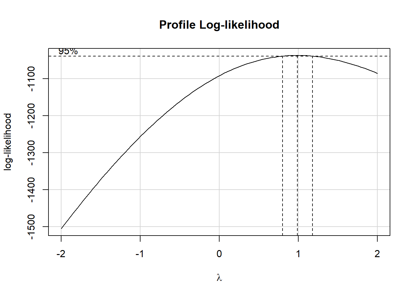

Since the recommended power transformation parameter \(\lambda\) is quite close to 1, we’ll not be using any transformation in this chapter.

20.4 The Full OLS model

model_parameters(fit1, ci = 0.95)

Parameter   | Coefficient |    SE |          95% CI | t(234) |      p
---------------------------------------------------------------------
(Intercept) |      -14.73 | 22.35 | [-58.77, 29.30] |  -0.66 | 0.510 
age         |        0.05 |  0.03 | [ -0.01,  0.11] |   1.53 | 0.128 
weight      |       -0.09 |  0.06 | [ -0.21,  0.04] |  -1.40 | 0.162 
height      |       -0.08 |  0.18 | [ -0.44,  0.27] |  -0.46 | 0.644 
neck        |       -0.48 |  0.23 | [ -0.94, -0.02] |  -2.06 | 0.040 
chest       |       -0.03 |  0.10 | [ -0.23,  0.18] |  -0.27 | 0.786 
abdomen     |        0.97 |  0.09 | [  0.79,  1.14] |  10.69 | < .001
hip         |       -0.21 |  0.15 | [ -0.50,  0.08] |  -1.45 | 0.148 
thigh       |        0.20 |  0.15 | [ -0.09,  0.49] |   1.36 | 0.176 
knee        |        0.04 |  0.25 | [ -0.45,  0.52] |   0.14 | 0.886 
ankle       |        0.17 |  0.22 | [ -0.27,  0.61] |   0.78 | 0.436 
biceps      |        0.16 |  0.17 | [ -0.18,  0.50] |   0.93 | 0.354 
forearm     |        0.44 |  0.20 | [  0.05,  0.83] |   2.21 | 0.028 
wrist       |       -1.59 |  0.53 | [ -2.64, -0.54] |  -2.98 | 0.003 

Uncertainty intervals (equal-tailed) and p-values (two-tailed) computed
  using a Wald t-distribution approximation.

check_model(fit1)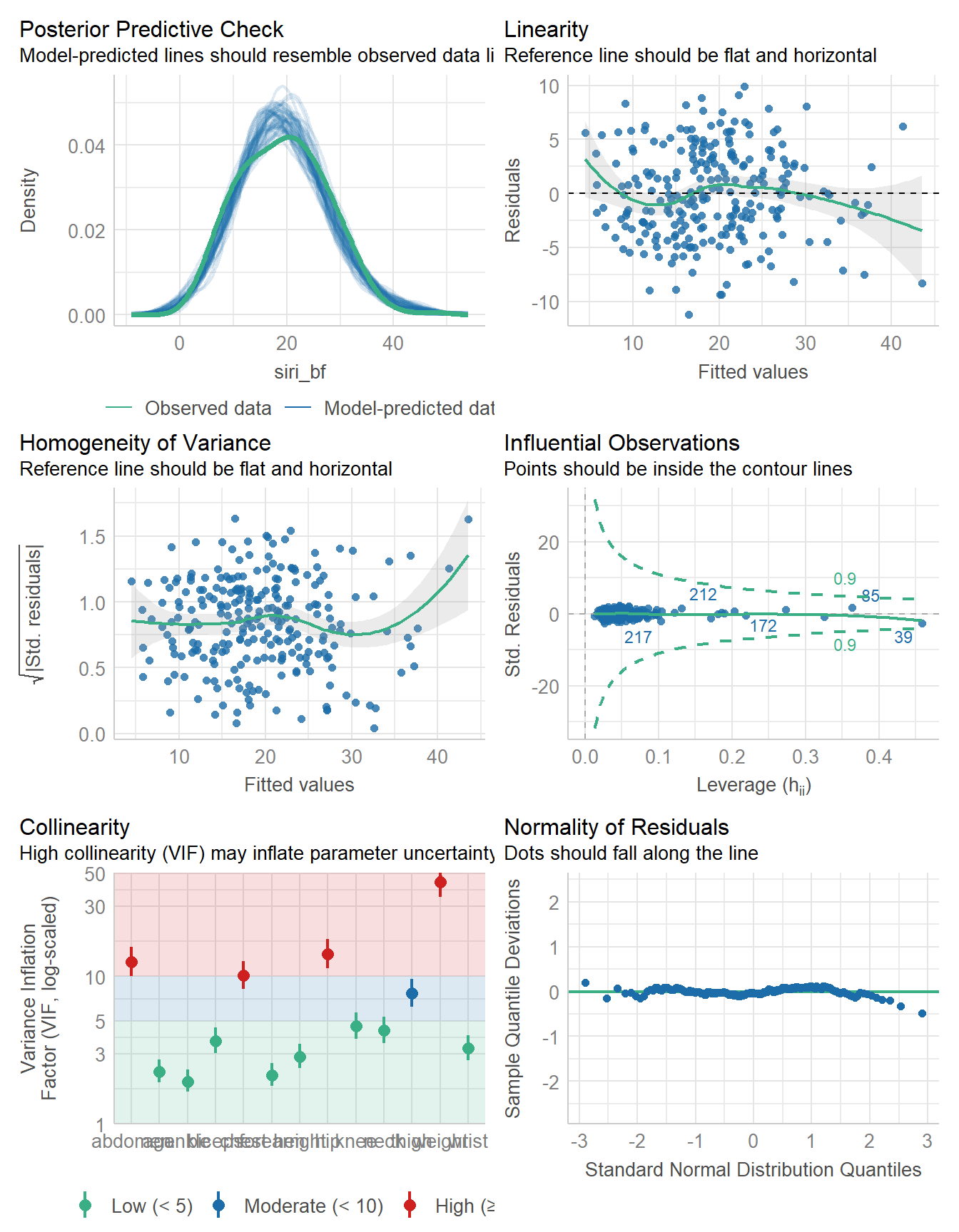

model_performance(fit1)

# Indices of model performance

AIC      |     AICc |      BIC |    R2 | R2 (adj.) |  RMSE | Sigma
------------------------------------------------------------------
1440.004 | 1442.073 | 1492.706 | 0.742 |     0.728 | 4.153 | 4.275

20.5 Identify a predictor subset with backwards stepwise elimination

fit2 <- select_parameters(fit1)

model_parameters(fit2, ci = 0.95)

Parameter   | Coefficient |    SE |          95% CI | t(239) |      p
---------------------------------------------------------------------
(Intercept) |      -19.90 | 11.68 | [-42.91,  3.11] |  -1.70 | 0.090 
age         |        0.05 |  0.03 | [ -0.01,  0.11] |   1.67 | 0.096 
weight      |       -0.09 |  0.04 | [ -0.17, -0.01] |  -2.21 | 0.028 
neck        |       -0.47 |  0.22 | [ -0.91, -0.03] |  -2.12 | 0.035 
abdomen     |        0.96 |  0.07 | [  0.82,  1.10] |  13.32 | < .001
hip         |       -0.21 |  0.14 | [ -0.48,  0.07] |  -1.49 | 0.136 
thigh       |        0.26 |  0.13 | [  0.00,  0.51] |   1.99 | 0.048 
forearm     |        0.49 |  0.19 | [  0.13,  0.86] |   2.65 | 0.008 
wrist       |       -1.46 |  0.51 | [ -2.47, -0.46] |  -2.88 | 0.004 

Uncertainty intervals (equal-tailed) and p-values (two-tailed) computed
  using a Wald t-distribution approximation.

compare_models(fit1, fit2)

Parameter    |                   fit1 |                   fit2
--------------------------------------------------------------
(Intercept)  | -14.73 (-58.77, 29.30) | -19.90 (-42.91,  3.11)
age          |   0.05 ( -0.01,  0.11) |   0.05 ( -0.01,  0.11)
weight       |  -0.09 ( -0.21,  0.04) |  -0.09 ( -0.17, -0.01)
neck         |  -0.48 ( -0.94, -0.02) |  -0.47 ( -0.91, -0.03)
abdomen      |   0.97 (  0.79,  1.14) |   0.96 (  0.82,  1.10)
hip          |  -0.21 ( -0.50,  0.08) |  -0.21 ( -0.48,  0.07)
thigh        |   0.20 ( -0.09,  0.49) |   0.26 (  0.00,  0.51)
forearm      |   0.44 (  0.05,  0.83) |   0.49 (  0.13,  0.86)
wrist        |  -1.59 ( -2.64, -0.54) |  -1.46 ( -2.47, -0.46)
chest        |  -0.03 ( -0.23,  0.18) |                       
ankle        |   0.17 ( -0.27,  0.61) |                       
height       |  -0.08 ( -0.44,  0.27) |                       
knee         |   0.04 ( -0.45,  0.52) |                       
biceps       |   0.16 ( -0.18,  0.50) |                       
--------------------------------------------------------------
Observations |                    248 |                    248

Note that fit2 drops five of the 13 predictors from the fit1 model.

check_model(fit2)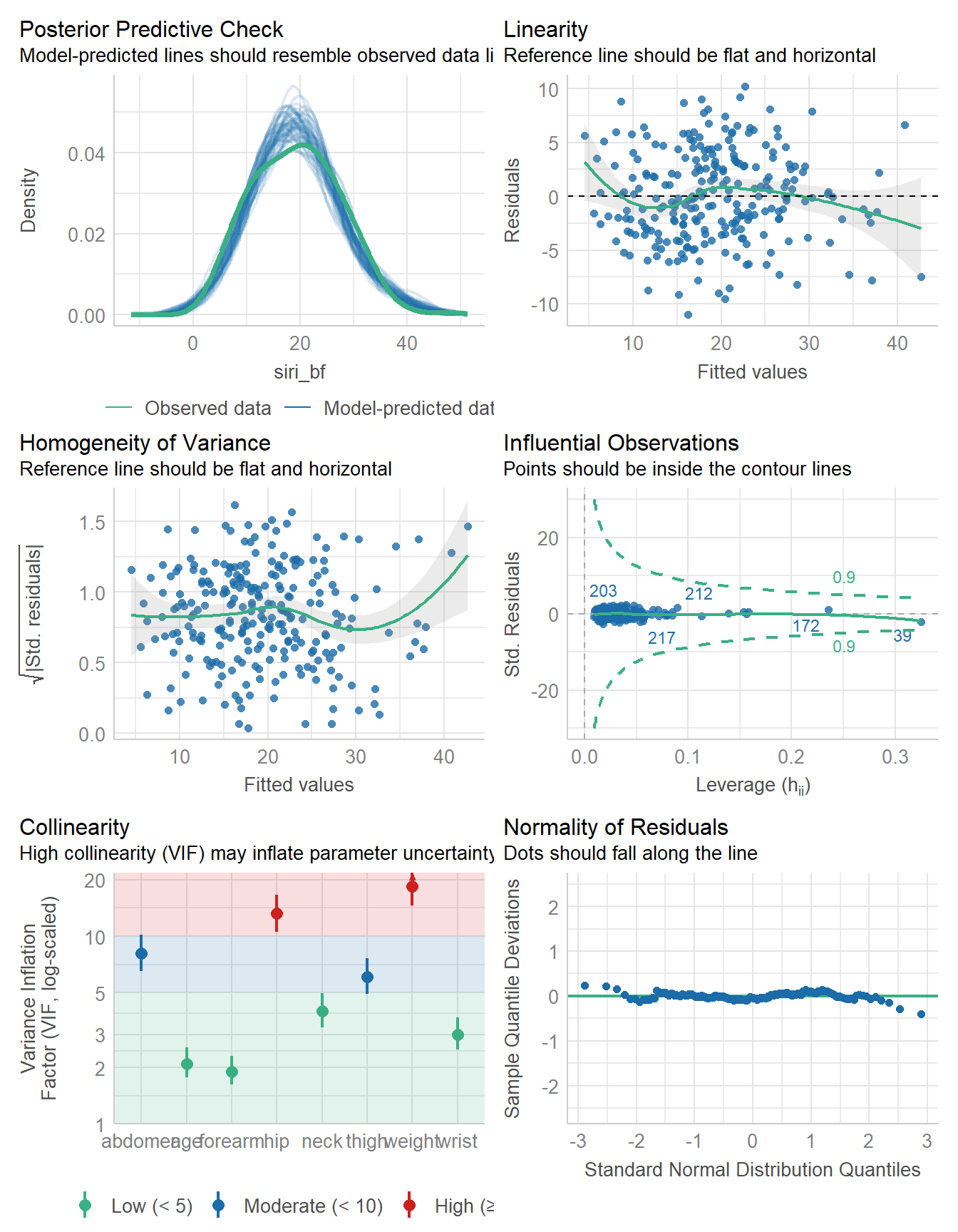

model_performance(fit2)

# Indices of model performance

AIC      |     AICc |      BIC |    R2 | R2 (adj.) |  RMSE | Sigma
------------------------------------------------------------------
1431.933 | 1432.861 | 1467.067 | 0.740 |     0.732 | 4.169 | 4.247

compare_performance(fit1, fit2)

# Comparison of Model Performance Indices

Name | Model |  AIC (weights) | AICc (weights) |  BIC (weights) |    R2 | R2 (adj.) |  RMSE | Sigma
---------------------------------------------------------------------------------------------------
fit1 |    lm | 1440.0 (0.017) | 1442.1 (0.010) | 1492.7 (<.001) | 0.742 |     0.728 | 4.153 | 4.275
fit2 |    lm | 1431.9 (0.983) | 1432.9 (0.990) | 1467.1 (>.999) | 0.740 |     0.732 | 4.169 | 4.247

plot(compare_performance(fit1, fit2))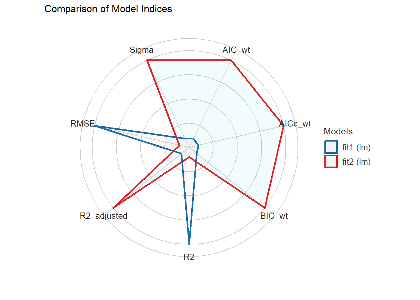

performance_mae(fit1)

[1] 3.418899

performance_mae(fit2)

[1] 3.412077

performance_rmse(fit1)

[1] 4.15292

performance_rmse(fit2)

[1] 4.169102

set.seed(431)
performance_accuracy(fit1, method = "cv", k = 5)

# Accuracy of Model Predictions

Accuracy (95% CI): 81.49% [73.12%, 92.09%]
Method: Correlation between observed and predicted

set.seed(431)
performance_accuracy(fit2, method = "cv", k = 5)

# Accuracy of Model Predictions

Accuracy (95% CI): 82.87% [74.24%, 93.11%]
Method: Correlation between observed and predicted

set.seed(431)
performance_cv(fit1)

# Cross-validation performance (30% holdout method)

MSE | RMSE |   R2
-----------------
16  |    4 | 0.74

set.seed(431)
performance_cv(fit2)

# Cross-validation performance (30% holdout method)

MSE | RMSE |   R2
-----------------
15  |  3.8 | 0.76

20.6 Best Subsets Regression and Mallows’ \(C_p\)

k <- ols_step_best_subset(fit1, 
                          max_order = 8,
                          metric = "cp")

k

                   Best Subsets Regression                    
--------------------------------------------------------------
Model Index    Predictors
--------------------------------------------------------------
     1         abdomen                                         
     2         weight abdomen                                  
     3         weight abdomen wrist                            
     4         weight abdomen forearm wrist                    
     5         weight neck abdomen forearm wrist               
     6         weight neck abdomen biceps forearm wrist        
     7         age weight neck abdomen thigh forearm wrist     
     8         age weight neck abdomen hip thigh forearm wrist 
--------------------------------------------------------------

                                                      Subsets Regression Summary                                                      
--------------------------------------------------------------------------------------------------------------------------------------
                       Adj.        Pred                                                                                                
Model    R-Square    R-Square    R-Square     C(p)         AIC         SBIC         SBC         MSEP         FPE       HSP       APC  
--------------------------------------------------------------------------------------------------------------------------------------
  1        0.6543      0.6529      0.6438    69.8409    1488.8082    784.0875    1499.3485    5783.2127    23.5075    0.0952    0.3513 
  2        0.7143      0.7120      0.7047    17.3601    1443.5224    739.4622    1457.5761    4798.8699    19.5840    0.0793    0.2927 
  3        0.7233      0.7199      0.7104    11.1761    1437.5707    733.6757    1455.1379    4666.5692    19.1197    0.0774    0.2857 
  4        0.7304      0.7259      0.7159     6.8132    1433.2074    729.5437    1454.2879    4567.1491    18.7863    0.0761    0.2807 
  5        0.7335      0.7280      0.7175     5.9241    1432.2633    728.7699    1456.8573    4531.9786    18.7150    0.0758    0.2797 
  6        0.7355      0.7290      0.7176     6.1051    1432.3916    729.0562    1460.4990    4516.6449    18.7247    0.0759    0.2798 
  7        0.7378      0.7302      0.7175     6.0319    1432.2408    729.1139    1463.8617    4496.3797    18.7135    0.0759    0.2797 
  8        0.7403      0.7316      0.7186     5.8272    1431.9331    729.0634    1467.0674    4473.4501    18.6905    0.0758    0.2793 
--------------------------------------------------------------------------------------------------------------------------------------
AIC: Akaike Information Criteria 
 SBIC: Sawa's Bayesian Information Criteria 
 SBC: Schwarz Bayesian Criteria 
 MSEP: Estimated error of prediction, assuming multivariate normality 
 FPE: Final Prediction Error 
 HSP: Hocking's Sp 
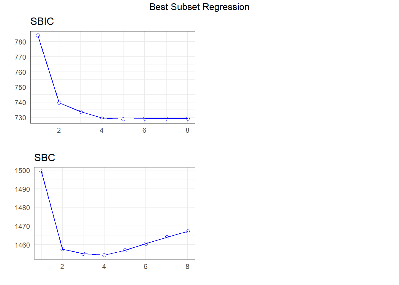
 APC: Amemiya Prediction Criteria 

plot(k)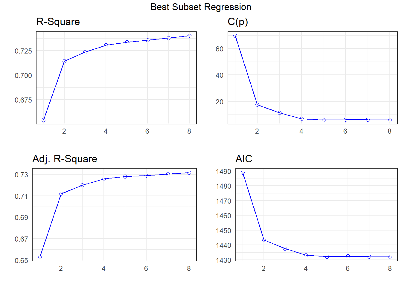

20.7 Four-Predictor Model

fit4 <- lm(
  siri_bf ~ weight + abdomen + forearm + wrist,
  data = bodyfat
) 

model_parameters(fit4, ci = 0.95)

Parameter   | Coefficient |   SE |           95% CI | t(243) |      p
---------------------------------------------------------------------
(Intercept) |      -33.61 | 7.26 | [-47.91, -19.32] |  -4.63 | < .001
weight      |       -0.14 | 0.02 | [ -0.19,  -0.09] |  -5.58 | < .001
abdomen     |        0.99 | 0.06 | [  0.88,   1.10] |  17.71 | < .001
forearm     |        0.45 | 0.18 | [  0.10,   0.81] |   2.51 | 0.013 
wrist       |       -1.48 | 0.44 | [ -2.36,  -0.61] |  -3.34 | < .001

Uncertainty intervals (equal-tailed) and p-values (two-tailed) computed
  using a Wald t-distribution approximation.

model_performance(fit4)

# Indices of model performance

AIC      |     AICc |      BIC |    R2 | R2 (adj.) |  RMSE | Sigma
------------------------------------------------------------------
1433.207 | 1433.556 | 1454.288 | 0.730 |     0.726 | 4.248 | 4.291

check_model(fit4)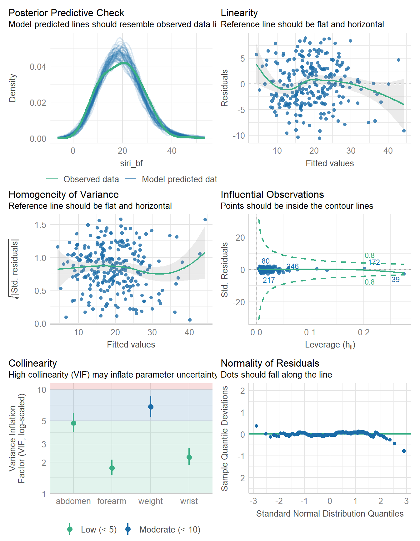

20.8 Five-Predictor Model

fit5 <- lm(
  siri_bf ~ weight + neck + abdomen + forearm + wrist,
  data = bodyfat
)

model_parameters(fit5, ci = 0.95)

Parameter   | Coefficient |   SE |           95% CI | t(242) |      p
---------------------------------------------------------------------
(Intercept) |      -29.23 | 7.67 | [-44.35, -14.11] |  -3.81 | < .001
weight      |       -0.12 | 0.03 | [ -0.17,  -0.07] |  -4.81 | < .001
neck        |       -0.37 | 0.22 | [ -0.81,   0.06] |  -1.70 | 0.090 
abdomen     |        1.00 | 0.06 | [  0.89,   1.11] |  17.85 | < .001
forearm     |        0.51 | 0.18 | [  0.15,   0.87] |   2.79 | 0.006 
wrist       |       -1.23 | 0.47 | [ -2.15,  -0.31] |  -2.62 | 0.009 

Uncertainty intervals (equal-tailed) and p-values (two-tailed) computed
  using a Wald t-distribution approximation.

model_performance(fit5)

# Indices of model performance

AIC      |     AICc |      BIC |    R2 | R2 (adj.) |  RMSE | Sigma
------------------------------------------------------------------
1432.263 | 1432.730 | 1456.857 | 0.734 |     0.728 | 4.223 | 4.275

check_model(fit5)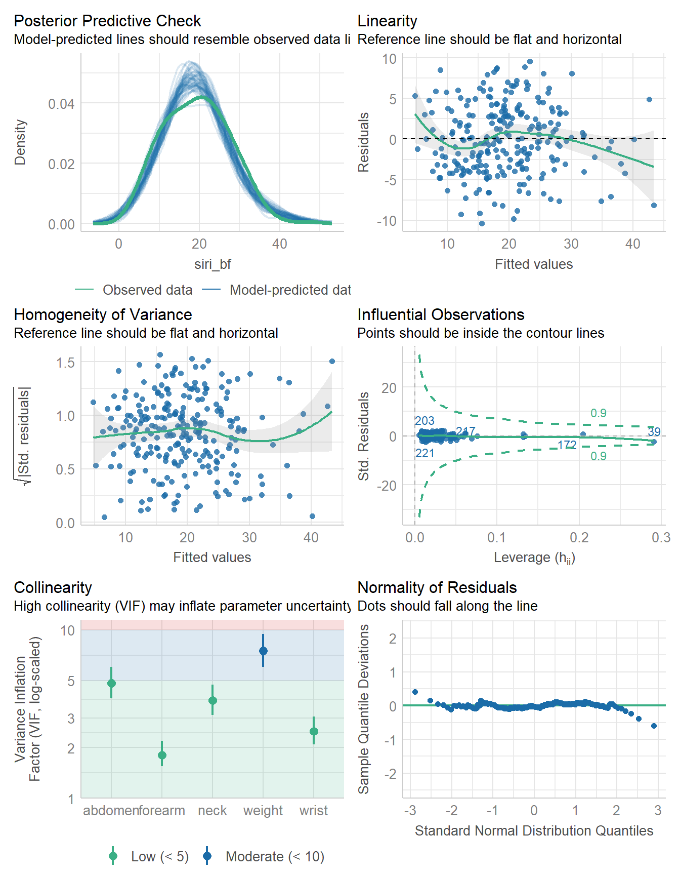

compare_performance(fit4, fit5)

# Comparison of Model Performance Indices

Name | Model |  AIC (weights) | AICc (weights) |  BIC (weights) |    R2 | R2 (adj.) |  RMSE | Sigma
---------------------------------------------------------------------------------------------------
fit4 |    lm | 1433.2 (0.384) | 1433.6 (0.398) | 1454.3 (0.783) | 0.730 |     0.726 | 4.248 | 4.291
fit5 |    lm | 1432.3 (0.616) | 1432.7 (0.602) | 1456.9 (0.217) | 0.734 |     0.728 | 4.223 | 4.275

set.seed(431)
performance_accuracy(fit1, method = "cv", k = 5)

# Accuracy of Model Predictions

Accuracy (95% CI): 81.49% [73.12%, 92.09%]
Method: Correlation between observed and predicted

set.seed(431)
performance_accuracy(fit2, method = "cv", k = 5)

# Accuracy of Model Predictions

Accuracy (95% CI): 82.87% [74.24%, 93.11%]
Method: Correlation between observed and predicted

set.seed(431)
performance_accuracy(fit4, method = "cv", k = 5)

# Accuracy of Model Predictions

Accuracy (95% CI): 83.10% [74.74%, 92.71%]
Method: Correlation between observed and predicted

set.seed(431)
performance_accuracy(fit5, method = "cv", k = 5)

# Accuracy of Model Predictions

Accuracy (95% CI): 82.99% [74.96%, 93.04%]
Method: Correlation between observed and predicted

set.seed(431)
performance_cv(fit1)

# Cross-validation performance (30% holdout method)

MSE | RMSE |   R2
-----------------
16  |    4 | 0.74

set.seed(431)
performance_cv(fit2)

# Cross-validation performance (30% holdout method)

MSE | RMSE |   R2
-----------------
15  |  3.8 | 0.76

set.seed(431)
performance_cv(fit4)

# Cross-validation performance (30% holdout method)

MSE | RMSE |   R2
-----------------
14  |  3.8 | 0.76

set.seed(431)
performance_cv(fit5)

# Cross-validation performance (30% holdout method)

MSE | RMSE |   R2
-----------------
15  |  3.9 | 0.75

20.9 Bayesian linear model

We’ll now refit the four-predictor model using stan_glm() and a weakly informative prior, as usual.

fit4b <- stan_glm(
  siri_bf ~ weight + abdomen + forearm + wrist,
  data = bodyfat, refresh = 0
) 

model_parameters(fit4b, ci = 0.95)

Parameter   | Median |           95% CI |     pd |  Rhat |     ESS |                   Prior
--------------------------------------------------------------------------------------------
(Intercept) | -33.40 | [-48.11, -19.22] |   100% | 1.003 | 2889.00 | Normal (19.28 +- 20.49)
weight      |  -0.14 | [ -0.19,  -0.09] |   100% | 1.004 | 2119.00 |   Normal (0.00 +- 0.71)
abdomen     |   0.99 | [  0.87,   1.10] |   100% | 1.002 | 2402.00 |   Normal (0.00 +- 1.92)
forearm     |   0.45 | [  0.09,   0.81] | 99.40% | 1.001 | 3820.00 |  Normal (0.00 +- 10.20)
wrist       |  -1.49 | [ -2.35,  -0.59] | 99.95% | 1.002 | 3160.00 |  Normal (0.00 +- 22.30)

Uncertainty intervals (equal-tailed) and p-values (two-tailed) computed
  using a MCMC distribution approximation.

model_performance(fit4b)

# Indices of model performance

ELPD     | ELPD_SE |    LOOIC | LOOIC_SE |     WAIC |    R2 | R2 (adj.) |  RMSE | Sigma
---------------------------------------------------------------------------------------
-717.386 |   9.726 | 1434.773 |   19.452 | 1434.619 | 0.727 |     0.716 | 4.248 | 4.300

check_model(fit4b)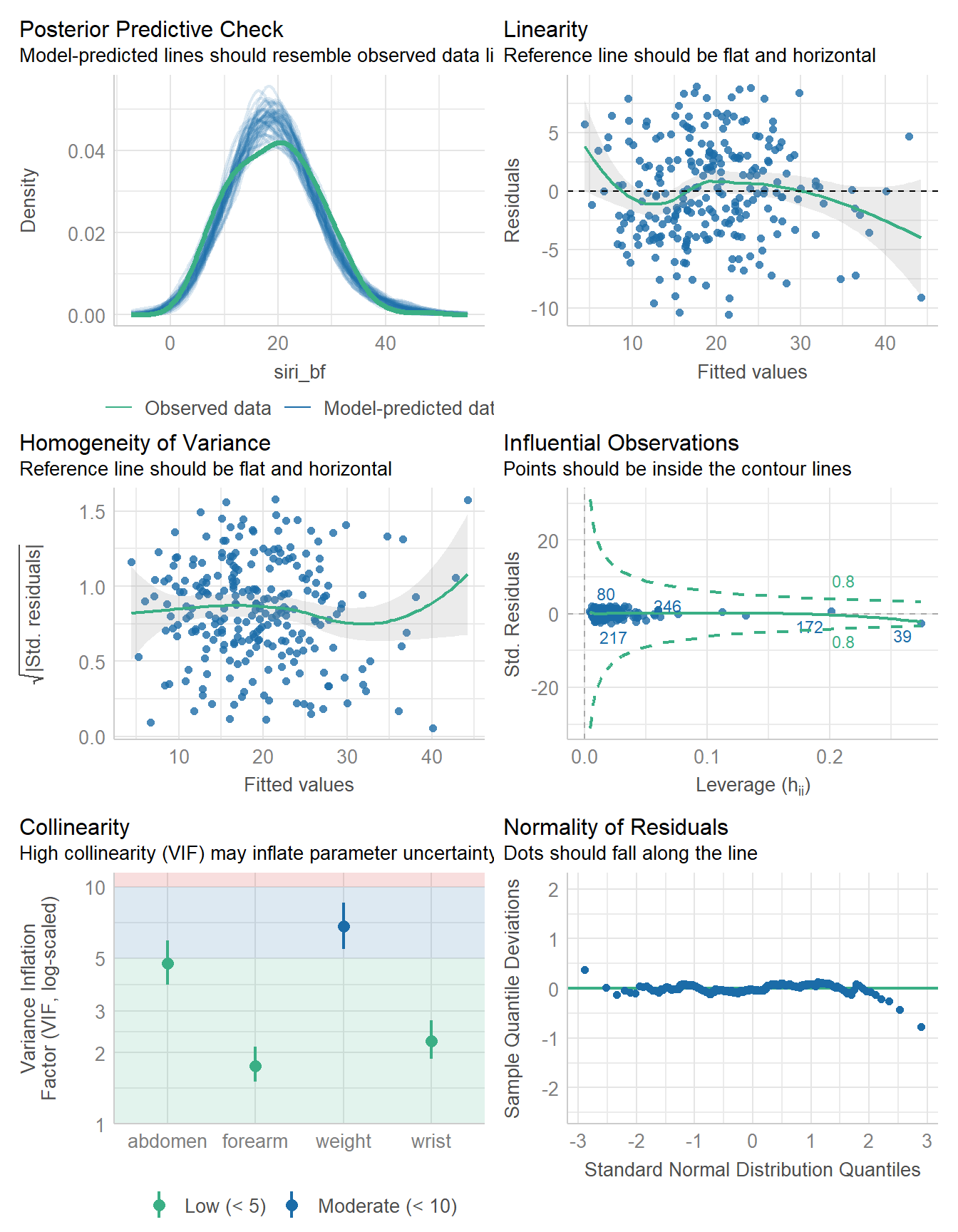

set.seed(431)
performance_accuracy(fit4b, method = "cv", k = 5)

# Accuracy of Model Predictions

Accuracy (95% CI): 83.11% [74.77%, 92.71%]
Method: Correlation between observed and predicted

set.seed(431)
performance_cv(fit4b)

# Cross-validation performance (30% holdout method)

MSE | RMSE |   R2
-----------------
14  |  3.8 | 0.76

20.10 For More Information

---

1. (Measurement standards are apparently those listed in Benhke and Wilmore (1974), pp. 45-48 where, for instance, the abdomen circumference is measured “laterally, at the level of the iliac crests, and anteriorly, at the umbilicus”.)

2. Siri’s equation is BF = 495/density - 450