21 Multiple Regression and Transformations
This is a sketchy draft with some useful content. I’ll remove this notice when I post a version of this Chapter that is essentially finished, but that won’t be until summer 2025.
21.1 R setup for this chapter
Appendix A lists all R packages used in this book, and also provides R session information. Appendix B describes the 431-Love.R script, and demonstrates its use.
21.2 Plasma Retinol and Beta-Carotene Dataset
Appendix C provides further guidance on pulling data from other systems into R, while Appendix D gives more information (including download links) for all data sets used in this book.
The data in this study come from an unpublished study related to Nierenberg et al. (1989). From Thérèse Stukel, one of the authors of that study, and posted to Statlib as well as Frank Harrell’s repository…
Observational studies have suggested that low dietary intake or low plasma concentrations of retinol, beta-carotene, or other carotenoids might be associated with increased risk of developing certain types of cancer. However, relatively few studies have investigated the determinants of plasma concentrations of these micronutrients. We designed a cross-sectional study to investigate the relationship between personal characteristics and dietary factors, and plasma concentrations of retinol, beta-carotene and other carotenoids. Study subjects (N = 315) were patients who had an elective surgical procedure during a three-year period to biopsy or remove a lesion of the lung, colon, breast, skin, ovary or uterus that was found to be non-cancerous. Plasma concentrations of the micronutrients varied widely from subject to subject.
21.2.1 Data Ingest
plasma <- read_csv("data/plasma.csv", show_col_types = FALSE) |>
  mutate(across(where(is.character), as_factor)) |>
  mutate(P_ID = as.character(P_ID)) |>
  janitor::clean_names()

plasma
# A tibble: 315 × 15
p_id age sex smokstat bmi vituse calories fat fiber alcohol
<chr> <dbl> <fct> <fct> <dbl> <fct> <dbl> <dbl> <dbl> <dbl>
1 1 64 Female Former 21.5 Fairly_Often 1299. 57 6.3 0
2 2 76 Female Never 23.9 Fairly_Often 1032. 50.1 15.8 0
3 3 38 Female Former 20.0 Not_Often 2372. 83.6 19.1 14.1
4 4 40 Female Former 25.1 Never 2450. 97.5 26.5 0.5
5 5 72 Female Never 21.0 Fairly_Often 1952. 82.6 16.2 0
6 6 40 Female Former 27.5 Never 1367. 56 9.6 1.3
7 7 65 Female Never 22.0 Not_Often 2214. 52 28.7 0
8 8 58 Female Never 28.8 Fairly_Often 1596. 63.4 10.9 0
9 9 35 Female Never 23.1 Never 1800. 57.8 20.3 0.6
10 10 55 Female Former 35.0 Never 1264. 39.6 15.5 0
# ℹ 305 more rows
# ℹ 5 more variables: cholesterol <dbl>, betadiet <dbl>, retdiet <dbl>,
# betaplasma <dbl>, retplasma <dbl>21.2.2 Variable Descriptions
| Variable | Description |
|---|---|
p_id |
Subject identification code |
age |
Age (years) |
sex |
Sex (Male, Female) |
smokstat |
Smoking status (Never, Former, Current Smoker) |
bmi |
Body mass index (weight/(height^2)) |
vituse |
Vitamin Use (Yes, fairly often; Yes, not often; No) |
calories |
Number of calories consumed per day. |
fat |
Grams of fat consumed per day. |
fiber |
Grams of fiber consumed per day. |
alcohol |
Number of alcoholic drinks consumed per week. |
cholesterol |
Cholesterol consumed (mg per day). |
betadiet |
Dietary beta-carotene consumed (mcg per day). |
retdiet |
Dietary retinol consumed (mcg per day) |
betaplasma |
Plasma beta-carotene (ng/ml) |
retplasma |
Plasma Retinol (ng/ml) |
n_miss(plasma)[1] 021.2.3 Data Summary; Outlier Removal
describe_distribution(plasma)Variable | Mean | SD | IQR | Range | Skewness | Kurtosis | n | n_Missing
-----------------------------------------------------------------------------------------------------
age | 50.15 | 14.58 | 24.00 | [19.00, 83.00] | 0.30 | -0.87 | 315 | 0
bmi | 26.16 | 6.01 | 7.16 | [16.33, 50.40] | 1.38 | 2.01 | 315 | 0
calories | 1796.65 | 680.35 | 772.60 | [445.20, 6662.20] | 1.75 | 8.13 | 315 | 0
fat | 77.03 | 33.83 | 41.40 | [14.40, 235.90] | 1.10 | 2.02 | 315 | 0
fiber | 12.79 | 5.33 | 6.50 | [3.10, 36.80] | 1.15 | 2.48 | 315 | 0
alcohol | 3.28 | 12.32 | 3.20 | [0.00, 203.00] | 13.82 | 221.33 | 315 | 0
cholesterol | 242.46 | 131.99 | 154.00 | [37.70, 900.70] | 1.48 | 3.41 | 315 | 0
betadiet | 2185.60 | 1473.89 | 1749.00 | [214.00, 9642.00] | 1.61 | 3.47 | 315 | 0
retdiet | 832.71 | 589.29 | 568.00 | [30.00, 6901.00] | 4.47 | 38.07 | 315 | 0
betaplasma | 189.89 | 183.00 | 142.00 | [0.00, 1415.00] | 3.56 | 17.21 | 315 | 0
retplasma | 602.79 | 208.90 | 253.00 | [179.00, 1727.00] | 1.31 | 4.02 | 315 | 0That alcohol value of 203 drinks per week is concerning.
# A tibble: 6 × 2
  alcohol     n
    <dbl> <int>
1    18.2     1
2    20       1
3    21       1
4    22       1
5    35       2
6   203       1
The next highest value is 35 drinks per week. I’m going to make the decision to remove this observation from the data, for the remainder of this chapter.
21.3 Predicting Plasma Beta-Carotene
Having removed the subject with an unrealistic alcohol value, our first main task is to predict betaplasma using (a subset of) most of the other variables in the data. Let’s look at that outcome.
p1 <- ggplot(plasma, aes(x = betaplasma)) +
  geom_histogram(bins = 15, fill = "blue", col = "white") +
  labs(
    x = "Plasma beta-carotene (ng/ml)",
    title = "Histogram"
  )

p2 <- ggplot(plasma, aes(sample = betaplasma)) +
  geom_qq() +
  geom_qq_line(col = "red") +
  labs(
    y = "Plasma beta-carotene",
    x = "Standard Normal Distribution",
    title = "Normal Q-Q plot"
  )

p3 <- ggplot(plasma, aes(x = betaplasma, y = "")) +
  geom_violin(fill = "cornsilk") +
  geom_boxplot(width = 0.2) +
  stat_summary(
    fun = mean, geom = "point",
    shape = 16, col = "red"
  ) +
  labs(
    y = "", x = "Plasma beta-carotene",
    title = "Boxplot with Violin"
  )

p1 + (p2 / p3 + plot_layout(heights = c(2, 1))) +
  plot_annotation(
    title = "Plasma Beta-Carotene in ng/ml"
  )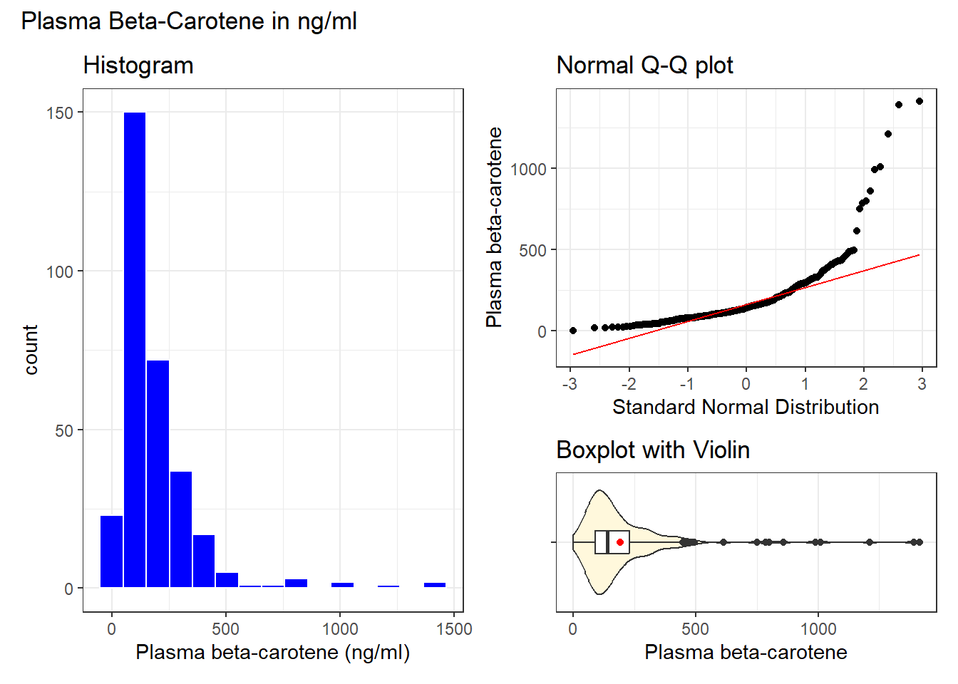
We see a fairly pronounced skew to the right here.
plasma |> reframe(lovedist(betaplasma))# A tibble: 1 × 10
n miss mean sd med mad min q25 q75 max
<int> <int> <dbl> <dbl> <dbl> <dbl> <dbl> <dbl> <dbl> <dbl>
1 314 0 190. 183. 140 88.2 0 89.5 230. 1415Note that we have a minimum value of 0 here. To use the Box-Cox method, we need to have values of our outcome that are strictly positive. The simplest solution to this problem (of seeing one or more zero values but no negative values) is to simply add one to each value of betaplasma before considering transformations.
fit0 <- lm((betaplasma + 1) ~ age + sex + smokstat + bmi + vituse +
  calories + fat + fiber + alcohol + cholesterol +
  betadiet, data = plasma)

boxCox(fit0)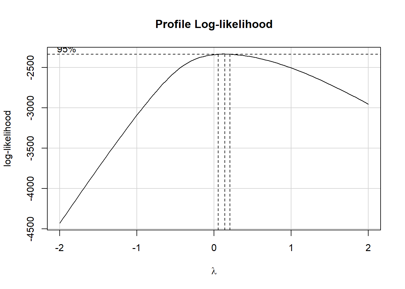
We’ll apply a logarithmic transformation to (betaplasma + 1) as our revised outcome for modeling.
p1 <- ggplot(plasma, aes(x = betaplasma)) +
  geom_histogram(bins = 20, fill = "coral", col = "blue")

p2 <- ggplot(plasma, aes(x = log(betaplasma + 1))) +
  geom_histogram(bins = 20, fill = "aquamarine", col = "blue")

p1 + p2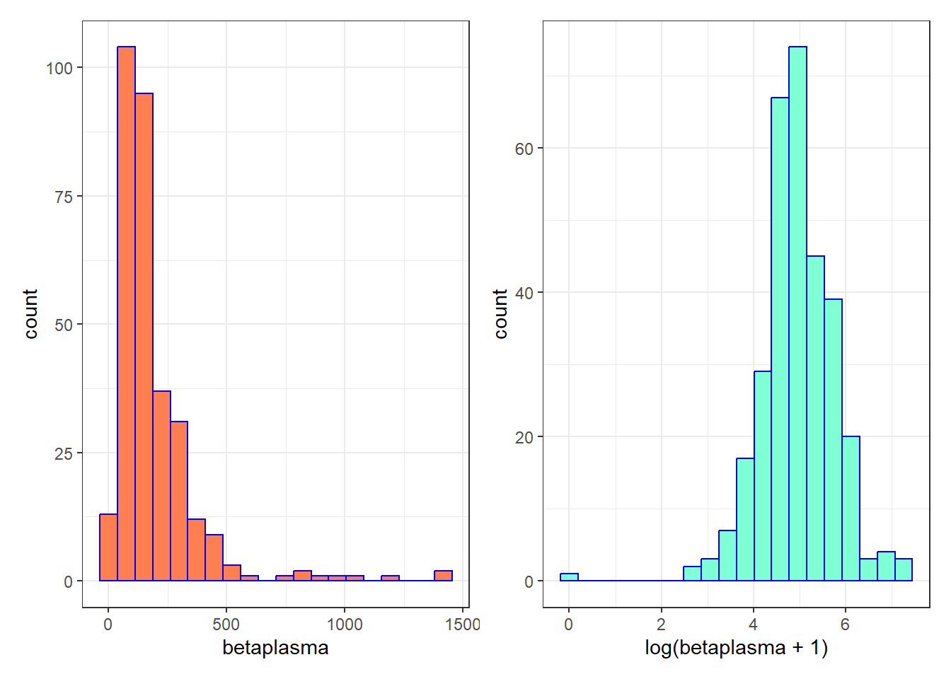
Most of our modeling of this transformed outcome is going to be affected, to some degree, by the outlying 0 value. Let’s take a closer look at that:
# A tibble: 6 × 2
  betaplasma     n
       <dbl> <int>
1          0     1
2         14     1
3         16     1
4         19     1
5         21     1
6         22     1
A value of 0 ng/ml for plasma beta-carotene also seems at best implausible. I’m going to go ahead and remove that subject from our study now, as well, and reframe our decision about a transformation accordingly.
plasma <- plasma |> filter(betaplasma > 0)21.3.1 Final Analytic Data (- 2 observations)
So now, having removed two observations:
- one for having an implausible level of
betaplasmaof 0 ng/ml, and - one for having an implausible level of
alcoholof 203 drinks per week,
we consider again the issue of transforming our outcome, and a Box-Cox plot, but now, thanks to dropping one of our outliers, we have a strictly positive set of betaplasma values to work with, so we no longer need to add 1 to that outcome.
fit00 <- lm(betaplasma ~
              age + sex + smokstat + bmi + vituse +
              calories + fat + fiber + alcohol +
              cholesterol + betadiet,
            data = plasma)

boxCox(fit00)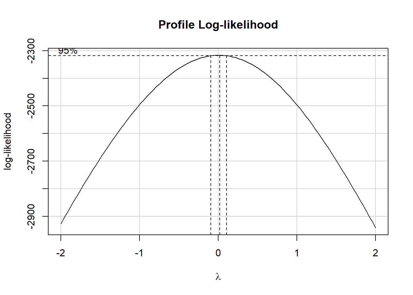
Again, we’re strongly encouraged to fit a logarithm of the outcome, by virtue of the estimated \(\lambda = 0\).
21.3.2 Initial OLS Fit
model_parameters(fit1)Parameter | Coefficient | SE | 95% CI | t(299) | p
------------------------------------------------------------------------------
(Intercept) | 5.48 | 0.28 | [ 4.93, 6.04] | 19.57 | < .001
age | 5.24e-03 | 2.94e-03 | [ 0.00, 0.01] | 1.78 | 0.076
sex [Male] | -0.23 | 0.13 | [-0.48, 0.02] | -1.85 | 0.066
smokstat [Never] | 0.09 | 0.08 | [-0.08, 0.25] | 1.02 | 0.308
smokstat [Current] | -0.21 | 0.12 | [-0.45, 0.04] | -1.66 | 0.098
bmi | -0.03 | 6.48e-03 | [-0.04, -0.02] | -4.87 | < .001
vituse [Not_Often] | -0.03 | 0.10 | [-0.22, 0.17] | -0.26 | 0.797
vituse [Never] | -0.30 | 0.09 | [-0.48, -0.12] | -3.25 | 0.001
calories | -2.19e-04 | 2.01e-04 | [ 0.00, 0.00] | -1.09 | 0.278
fat | 1.40e-03 | 3.18e-03 | [ 0.00, 0.01] | 0.44 | 0.659
fiber | 0.03 | 0.01 | [ 0.01, 0.05] | 2.78 | 0.006
alcohol | 5.25e-03 | 8.76e-03 | [-0.01, 0.02] | 0.60 | 0.549
cholesterol | -2.70e-04 | 4.38e-04 | [ 0.00, 0.00] | -0.62 | 0.538
betadiet | 4.69e-05 | 2.95e-05 | [ 0.00, 0.00] | 1.59 | 0.113
Uncertainty intervals (equal-tailed) and p-values (two-tailed) computed
using a Wald t-distribution approximation.model_performance(fit1)# Indices of model performance
AIC | AICc | BIC | R2 | R2 (adj.) | RMSE | Sigma
---------------------------------------------------------------
646.464 | 648.080 | 702.657 | 0.249 | 0.216 | 0.648 | 0.663check_model(fit1)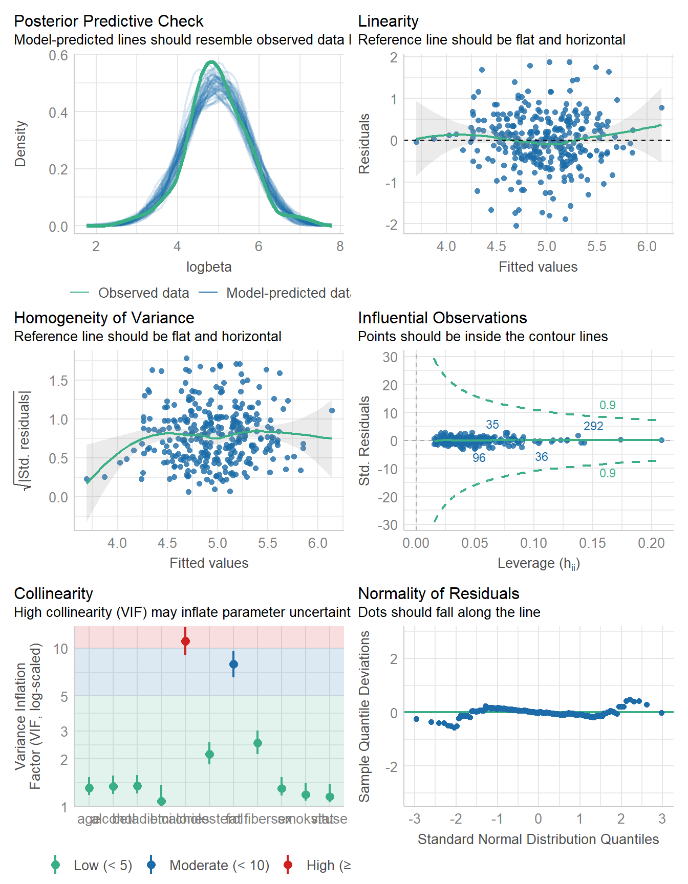
21.3.3 Best Subsets Suggestion?
k <- ols_step_best_subset(fit1,
                          max_order = 11,
                          metric = "cp")
k Best Subsets Regression
------------------------------------------------------------------------------------------
Model Index Predictors
------------------------------------------------------------------------------------------
1 bmi
2 bmi vituse
3 bmi vituse fiber
4 bmi vituse calories fiber
5 smokstat bmi vituse calories fiber
6 smokstat bmi vituse calories fiber betadiet
7 age sex smokstat bmi vituse calories fiber
8 age sex smokstat bmi vituse calories fiber betadiet
9 age sex smokstat bmi vituse calories fiber cholesterol betadiet
10 age sex smokstat bmi vituse calories fiber alcohol cholesterol betadiet
11 age sex smokstat bmi vituse calories fat fiber alcohol cholesterol betadiet
------------------------------------------------------------------------------------------
Subsets Regression Summary
-----------------------------------------------------------------------------------------------------------------------------------
Adj. Pred
Model R-Square R-Square R-Square C(p) AIC SBIC SBC MSEP FPE HSP APC
-----------------------------------------------------------------------------------------------------------------------------------
1 0.0790 0.0760 0.0672 57.5387 686.2096 -202.6728 697.4483 162.0541 0.5211 0.0017 0.9329
2 0.1327 0.1243 0.111 40.1581 671.3979 -219.4340 690.1289 153.0952 0.4954 0.0016 0.8841
3 0.1708 0.1600 0.1438 26.9872 659.3289 -231.3437 681.8061 146.8413 0.4767 0.0015 0.8507
4 0.2062 0.1933 0.175 14.8858 647.6592 -242.6879 673.8826 141.0242 0.4592 0.0015 0.8195
5 0.2254 0.2077 0.1839 11.2438 643.9939 -248.0769 677.7098 138.0622 0.4525 0.0015 0.8048
6 0.2332 0.2130 0.1862 10.1707 642.8577 -249.0400 680.3197 137.1339 0.4508 0.0014 0.8019
7 0.2403 0.2177 0.1883 9.3375 641.9383 -249.7554 683.1465 136.3077 0.4495 0.0014 0.7996
8 0.2466 0.2217 0.189 8.8230 641.3242 -250.1441 686.2786 135.6201 0.4487 0.0014 0.7980
9 0.2476 0.2201 0.1847 10.4380 642.9220 -248.4318 691.6227 135.8945 0.4510 0.0014 0.8021
10 0.2482 0.2181 0.18 12.1951 644.6680 -246.5767 697.1149 136.2354 0.4535 0.0015 0.8066
11 0.2487 0.2160 0.1738 14.0000 646.4639 -244.6723 702.6569 136.6003 0.4561 0.0015 0.8112
-----------------------------------------------------------------------------------------------------------------------------------
AIC: Akaike Information Criteria
SBIC: Sawa's Bayesian Information Criteria
SBC: Schwarz Bayesian Criteria
MSEP: Estimated error of prediction, assuming multivariate normality
FPE: Final Prediction Error
HSP: Hocking's Sp
APC: Amemiya Prediction Criteria plot(k)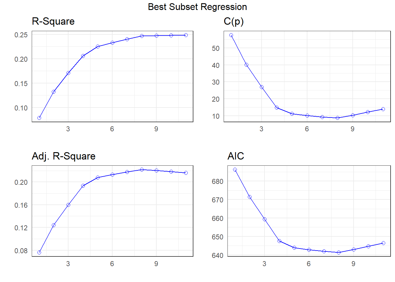
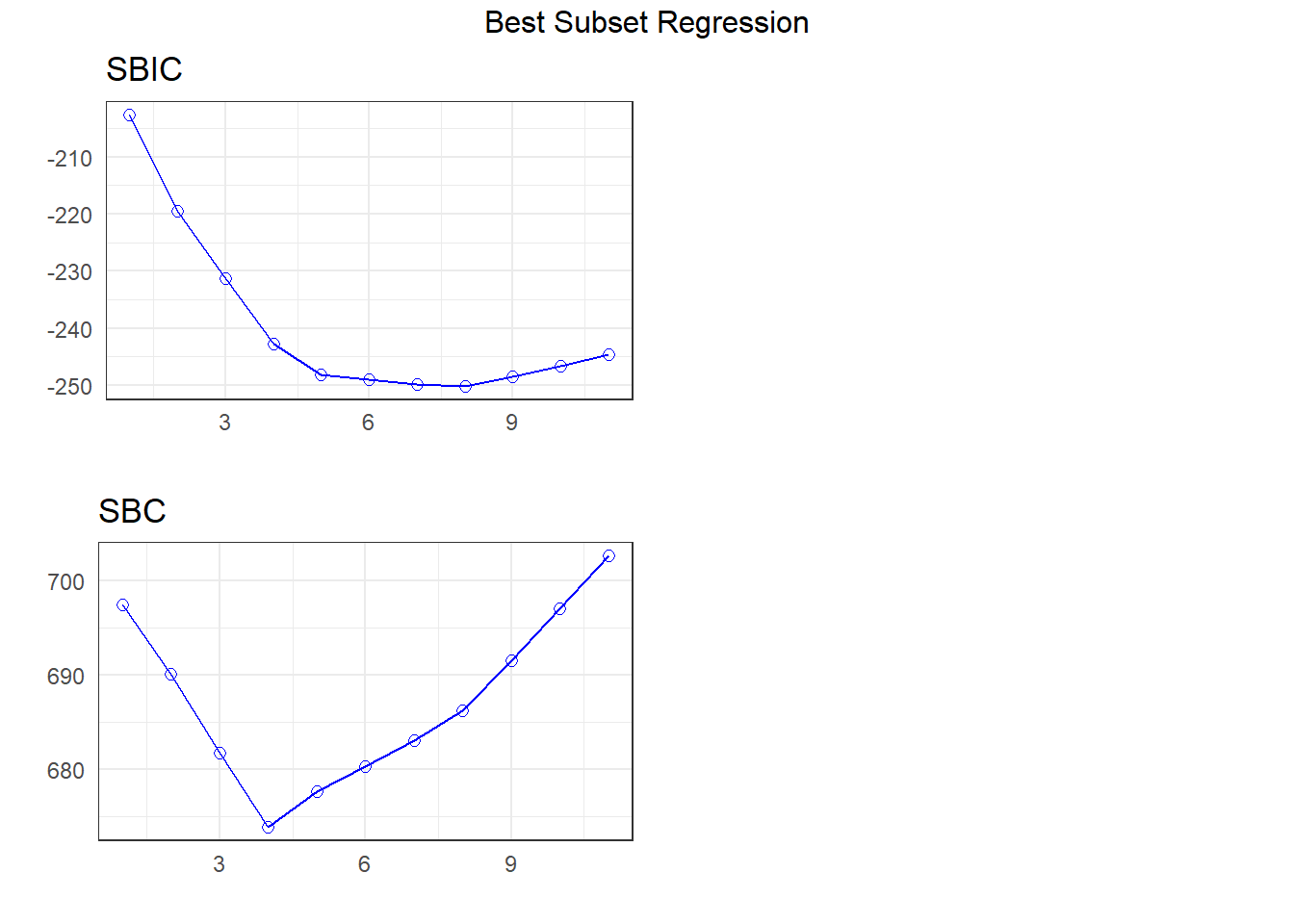
I’m going to look more closely at the four-predictor (suggested by SBC) and eight-predictor (suggested by \(C_p\)) subsets1
21.3.4 Four-Predictor Model
fit4 <- lm(logbeta ~ bmi + vituse + calories + fiber,
data = plasma)compare_models(fit1, fit4)Parameter | fit1 | fit4
------------------------------------------------------------------------
(Intercept) | 5.48 ( 4.93, 6.04) | 5.79 ( 5.37, 6.21)
bmi | -0.03 (-0.04, -0.02) | -0.03 (-0.04, -0.02)
vituse [Not_Often] | -0.03 (-0.22, 0.17) | -0.07 (-0.26, 0.12)
vituse [Never] | -0.30 (-0.48, -0.12) | -0.36 (-0.53, -0.18)
calories | -2.19e-04 ( 0.00, 0.00) | -2.66e-04 ( 0.00, 0.00)
fiber | 0.03 ( 0.01, 0.05) | 0.04 ( 0.03, 0.06)
smokstat [Current] | -0.21 (-0.45, 0.04) |
age | 5.24e-03 ( 0.00, 0.01) |
sex [Male] | -0.23 (-0.48, 0.02) |
smokstat [Never] | 0.09 (-0.08, 0.25) |
cholesterol | -2.70e-04 ( 0.00, 0.00) |
fat | 1.40e-03 ( 0.00, 0.01) |
alcohol | 5.25e-03 (-0.01, 0.02) |
betadiet | 4.69e-05 ( 0.00, 0.00) |
------------------------------------------------------------------------
Observations | 313 | 313model_parameters(fit4, ci = 0.95)Parameter | Coefficient | SE | 95% CI | t(307) | p
------------------------------------------------------------------------------
(Intercept) | 5.79 | 0.21 | [ 5.37, 6.21] | 27.17 | < .001
bmi | -0.03 | 6.38e-03 | [-0.04, -0.02] | -4.63 | < .001
vituse [Not_Often] | -0.07 | 0.10 | [-0.26, 0.12] | -0.69 | 0.493
vituse [Never] | -0.36 | 0.09 | [-0.53, -0.18] | -3.99 | < .001
calories | -2.66e-04 | 7.19e-05 | [ 0.00, 0.00] | -3.70 | < .001
fiber | 0.04 | 8.41e-03 | [ 0.03, 0.06] | 5.21 | < .001
Uncertainty intervals (equal-tailed) and p-values (two-tailed) computed
using a Wald t-distribution approximation.model_performance(fit4)# Indices of model performance
AIC | AICc | BIC | R2 | R2 (adj.) | RMSE | Sigma
---------------------------------------------------------------
647.659 | 648.026 | 673.883 | 0.206 | 0.193 | 0.666 | 0.672check_model(fit4)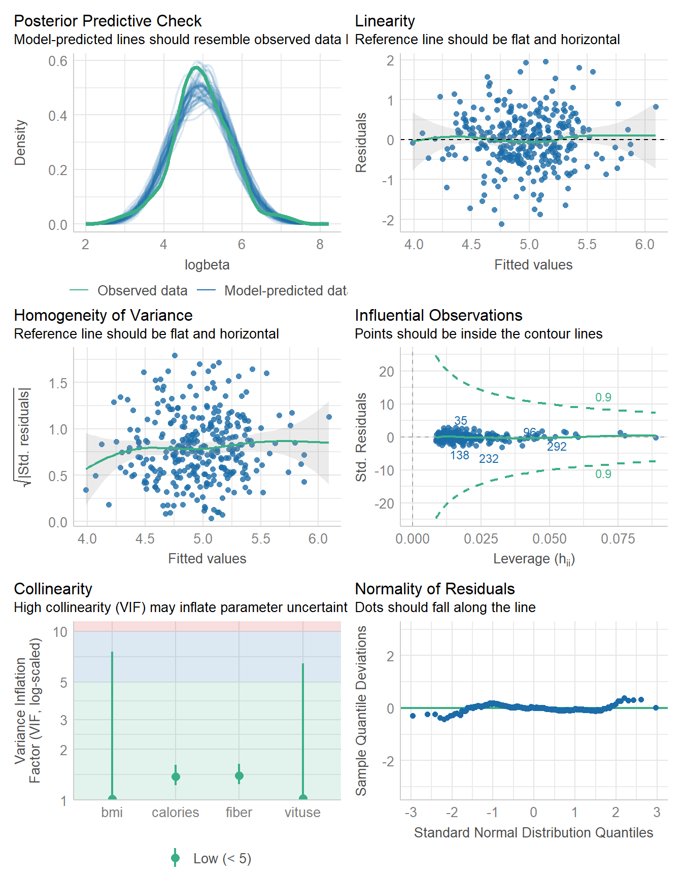
21.3.5 Eight-Predictor Model
fit8 <- lm(logbeta ~ age + sex + smokstat + bmi +
             vituse + calories + fiber + betadiet,
data = plasma)compare_models(fit1, fit8)Parameter | fit1 | fit8
------------------------------------------------------------------------
(Intercept) | 5.48 ( 4.93, 6.04) | 5.49 ( 4.95, 6.04)
age | 5.24e-03 ( 0.00, 0.01) | 5.40e-03 ( 0.00, 0.01)
sex [Male] | -0.23 (-0.48, 0.02) | -0.23 (-0.48, 0.01)
smokstat [Never] | 0.09 (-0.08, 0.25) | 0.08 (-0.09, 0.24)
smokstat [Current] | -0.21 (-0.45, 0.04) | -0.21 (-0.46, 0.03)
bmi | -0.03 (-0.04, -0.02) | -0.03 (-0.05, -0.02)
vituse [Not_Often] | -0.03 (-0.22, 0.17) | -0.02 (-0.21, 0.17)
vituse [Never] | -0.30 (-0.48, -0.12) | -0.29 (-0.46, -0.11)
calories | -2.19e-04 ( 0.00, 0.00) | -1.70e-04 ( 0.00, 0.00)
fiber | 0.03 ( 0.01, 0.05) | 0.03 ( 0.01, 0.05)
betadiet | 4.69e-05 ( 0.00, 0.00) | 4.65e-05 ( 0.00, 0.00)
cholesterol | -2.70e-04 ( 0.00, 0.00) |
fat | 1.40e-03 ( 0.00, 0.01) |
alcohol | 5.25e-03 (-0.01, 0.02) |
------------------------------------------------------------------------
Observations | 313 | 313model_parameters(fit8)Parameter | Coefficient | SE | 95% CI | t(302) | p
------------------------------------------------------------------------------
(Intercept) | 5.49 | 0.28 | [ 4.95, 6.04] | 19.90 | < .001
age | 5.40e-03 | 2.90e-03 | [ 0.00, 0.01] | 1.86 | 0.063
sex [Male] | -0.23 | 0.12 | [-0.48, 0.01] | -1.92 | 0.056
smokstat [Never] | 0.08 | 0.08 | [-0.09, 0.24] | 0.94 | 0.350
smokstat [Current] | -0.21 | 0.12 | [-0.46, 0.03] | -1.75 | 0.081
bmi | -0.03 | 6.35e-03 | [-0.05, -0.02] | -5.13 | < .001
vituse [Not_Often] | -0.02 | 0.10 | [-0.21, 0.17] | -0.24 | 0.814
vituse [Never] | -0.29 | 0.09 | [-0.46, -0.11] | -3.21 | 0.001
calories | -1.70e-04 | 7.71e-05 | [ 0.00, 0.00] | -2.21 | 0.028
fiber | 0.03 | 9.36e-03 | [ 0.01, 0.05] | 3.13 | 0.002
betadiet | 4.65e-05 | 2.92e-05 | [ 0.00, 0.00] | 1.59 | 0.113
Uncertainty intervals (equal-tailed) and p-values (two-tailed) computed
using a Wald t-distribution approximation.model_performance(fit8)# Indices of model performance
AIC | AICc | BIC | R2 | R2 (adj.) | RMSE | Sigma
---------------------------------------------------------------
641.324 | 642.364 | 686.279 | 0.247 | 0.222 | 0.649 | 0.660check_model(fit8)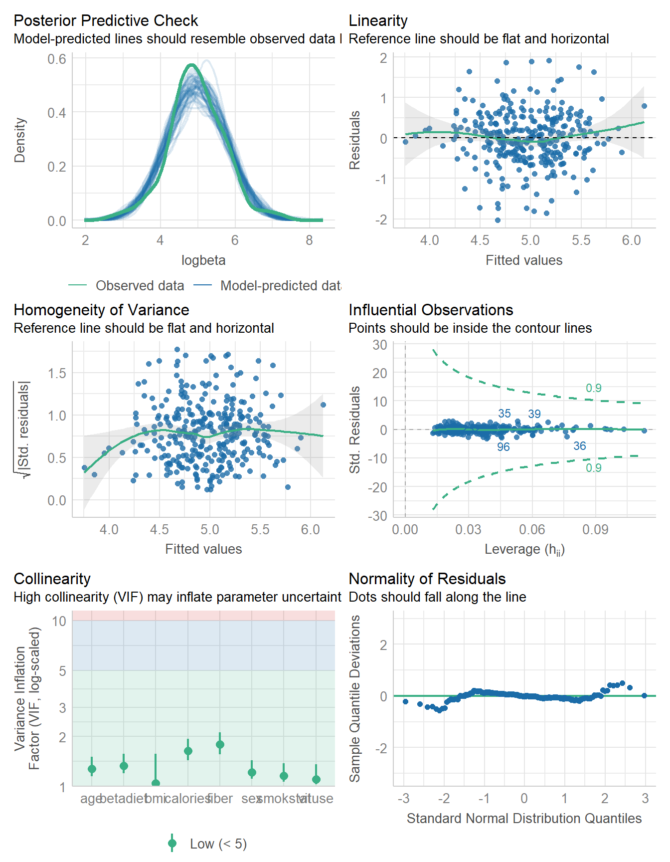
21.3.6 Our Three Models So Far
compare_performance(fit1, fit4, fit8)# Comparison of Model Performance Indices
Name | Model | AIC (weights) | AICc (weights) | BIC (weights) | R2 | R2 (adj.) | RMSE | Sigma
-------------------------------------------------------------------------------------------------
fit1 | lm | 646.5 (0.068) | 648.1 (0.051) | 702.7 (<.001) | 0.249 | 0.216 | 0.648 | 0.663
fit4 | lm | 647.7 (0.038) | 648.0 (0.053) | 673.9 (0.998) | 0.206 | 0.193 | 0.666 | 0.672
fit8 | lm | 641.3 (0.894) | 642.4 (0.896) | 686.3 (0.002) | 0.247 | 0.222 | 0.649 | 0.660plot(compare_performance(fit1, fit4, fit8))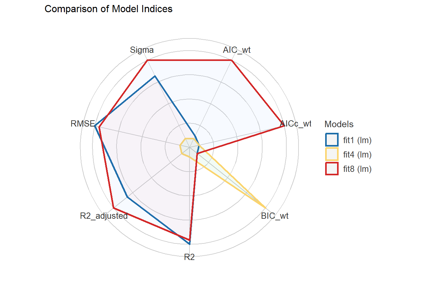
set.seed(431)
performance_accuracy(fit1, method = "cv", k = 5)
# Accuracy of Model Predictions
Accuracy (95% CI): 42.42% [32.42%, 52.44%]
Method: Correlation between observed and predictedset.seed(431)
performance_accuracy(fit4, method = "cv", k = 5)# Accuracy of Model Predictions
Accuracy (95% CI): 42.98% [37.50%, 52.45%]
Method: Correlation between observed and predictedset.seed(431)
performance_accuracy(fit8, method = "cv", k = 5)# Accuracy of Model Predictions
Accuracy (95% CI): 44.05% [32.92%, 57.60%]
Method: Correlation between observed and predictedset.seed(431)
performance_cv(fit1)# Cross-validation performance (30% holdout method)
MSE | RMSE | R2
------------------
0.56 | 0.75 | 0.19set.seed(431)
performance_cv(fit4)# Cross-validation performance (30% holdout method)
MSE | RMSE | R2
------------------
0.56 | 0.75 | 0.19set.seed(431)
performance_cv(fit8)# Cross-validation performance (30% holdout method)
MSE | RMSE | R2
------------------
0.55 | 0.74 | 0.2121.4 Using the Lasso
Need to discuss glmnet package, and point to:
- https://rpubs.com/jmkelly91/881590
- https://glmnet.stanford.edu/articles/glmnet.html#linear-regression-family-gaussian-default
and add some of the comments I used in https://thomaselove.github.io/432-notes/lasso.html#using-the-lasso-to-suggest-a-smaller-model
pred_x <- model.matrix(fit1)
out_y <- plasma |> select(logbeta) |> as.matrix()

set.seed(431)
lasso <- cv.glmnet(x = pred_x, y = out_y,
                   type.measure = "mse",
                   alpha = 1, family = "gaussian",
nlambda = 200, nfolds = 10)plot(lasso)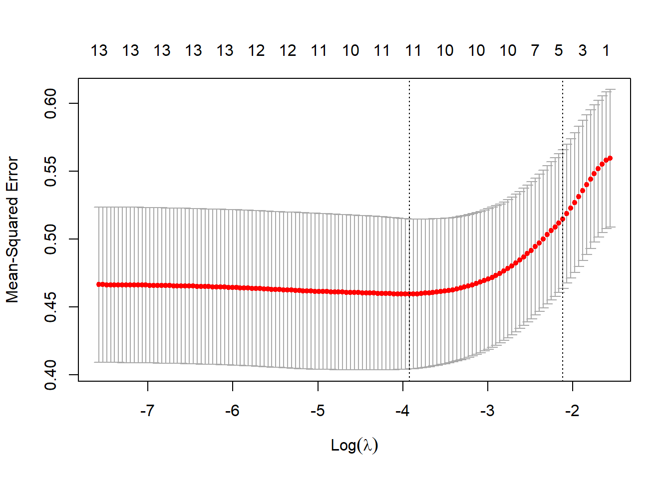
log(lasso$lambda.min)[1] -3.921033predict(lasso, type = "coef", s = "lambda.min")15 x 1 sparse Matrix of class "dgCMatrix"
lambda.min
(Intercept) 5.423141e+00
(Intercept) .
age 4.601321e-03
sexMale -1.703956e-01
smokstatNever 6.368383e-02
smokstatCurrent -1.874663e-01
bmi -2.918528e-02
vituseNot_Often .
vituseNever -2.486722e-01
calories -5.125006e-05
fat -4.158782e-04
fiber 2.216516e-02
alcohol .
cholesterol -3.158420e-04
betadiet 4.038103e-05We can use the lasso to identify a set of predictors to drop. Here, the lasso only drops the alcohol variable from our initial set of predictors, since we aren’t willing to drop just one level of a multi-categorical predictor like vituse.
21.4.1 No “alcohol” model
fit10 <- lm(logbeta ~ age + sex + smokstat + bmi +
             vituse + calories + fat + fiber +
             cholesterol + betadiet,
data = plasma)compare_models(fit1, fit10)Parameter | fit1 | fit10
------------------------------------------------------------------------
(Intercept) | 5.48 ( 4.93, 6.04) | 5.49 ( 4.94, 6.04)
age | 5.24e-03 ( 0.00, 0.01) | 5.35e-03 ( 0.00, 0.01)
sex [Male] | -0.23 (-0.48, 0.02) | -0.22 (-0.46, 0.02)
smokstat [Never] | 0.09 (-0.08, 0.25) | 0.08 (-0.09, 0.24)
smokstat [Current] | -0.21 (-0.45, 0.04) | -0.21 (-0.45, 0.03)
bmi | -0.03 (-0.04, -0.02) | -0.03 (-0.04, -0.02)
vituse [Not_Often] | -0.03 (-0.22, 0.17) | -0.02 (-0.21, 0.17)
vituse [Never] | -0.30 (-0.48, -0.12) | -0.29 (-0.47, -0.11)
calories | -2.19e-04 ( 0.00, 0.00) | -1.73e-04 ( 0.00, 0.00)
fat | 1.40e-03 ( 0.00, 0.01) | 8.53e-04 (-0.01, 0.01)
fiber | 0.03 ( 0.01, 0.05) | 0.03 ( 0.01, 0.05)
cholesterol | -2.70e-04 ( 0.00, 0.00) | -2.90e-04 ( 0.00, 0.00)
betadiet | 4.69e-05 ( 0.00, 0.00) | 4.81e-05 ( 0.00, 0.00)
alcohol | 5.25e-03 (-0.01, 0.02) |
------------------------------------------------------------------------
Observations | 313 | 313model_parameters(fit10)Parameter | Coefficient | SE | 95% CI | t(300) | p
------------------------------------------------------------------------------
(Intercept) | 5.49 | 0.28 | [ 4.94, 6.04] | 19.66 | < .001
age | 5.35e-03 | 2.94e-03 | [ 0.00, 0.01] | 1.82 | 0.069
sex [Male] | -0.22 | 0.12 | [-0.46, 0.02] | -1.77 | 0.078
smokstat [Never] | 0.08 | 0.08 | [-0.09, 0.24] | 0.95 | 0.343
smokstat [Current] | -0.21 | 0.12 | [-0.45, 0.03] | -1.72 | 0.087
bmi | -0.03 | 6.40e-03 | [-0.04, -0.02] | -5.02 | < .001
vituse [Not_Often] | -0.02 | 0.10 | [-0.21, 0.17] | -0.21 | 0.834
vituse [Never] | -0.29 | 0.09 | [-0.47, -0.11] | -3.20 | 0.002
calories | -1.73e-04 | 1.86e-04 | [ 0.00, 0.00] | -0.93 | 0.353
fat | 8.53e-04 | 3.04e-03 | [-0.01, 0.01] | 0.28 | 0.779
fiber | 0.03 | 0.01 | [ 0.01, 0.05] | 2.72 | 0.007
cholesterol | -2.90e-04 | 4.36e-04 | [ 0.00, 0.00] | -0.66 | 0.507
betadiet | 4.81e-05 | 2.94e-05 | [ 0.00, 0.00] | 1.64 | 0.103
Uncertainty intervals (equal-tailed) and p-values (two-tailed) computed
using a Wald t-distribution approximation.model_performance(fit10)# Indices of model performance
AIC | AICc | BIC | R2 | R2 (adj.) | RMSE | Sigma
---------------------------------------------------------------
644.840 | 646.249 | 697.287 | 0.248 | 0.218 | 0.648 | 0.662check_model(fit10)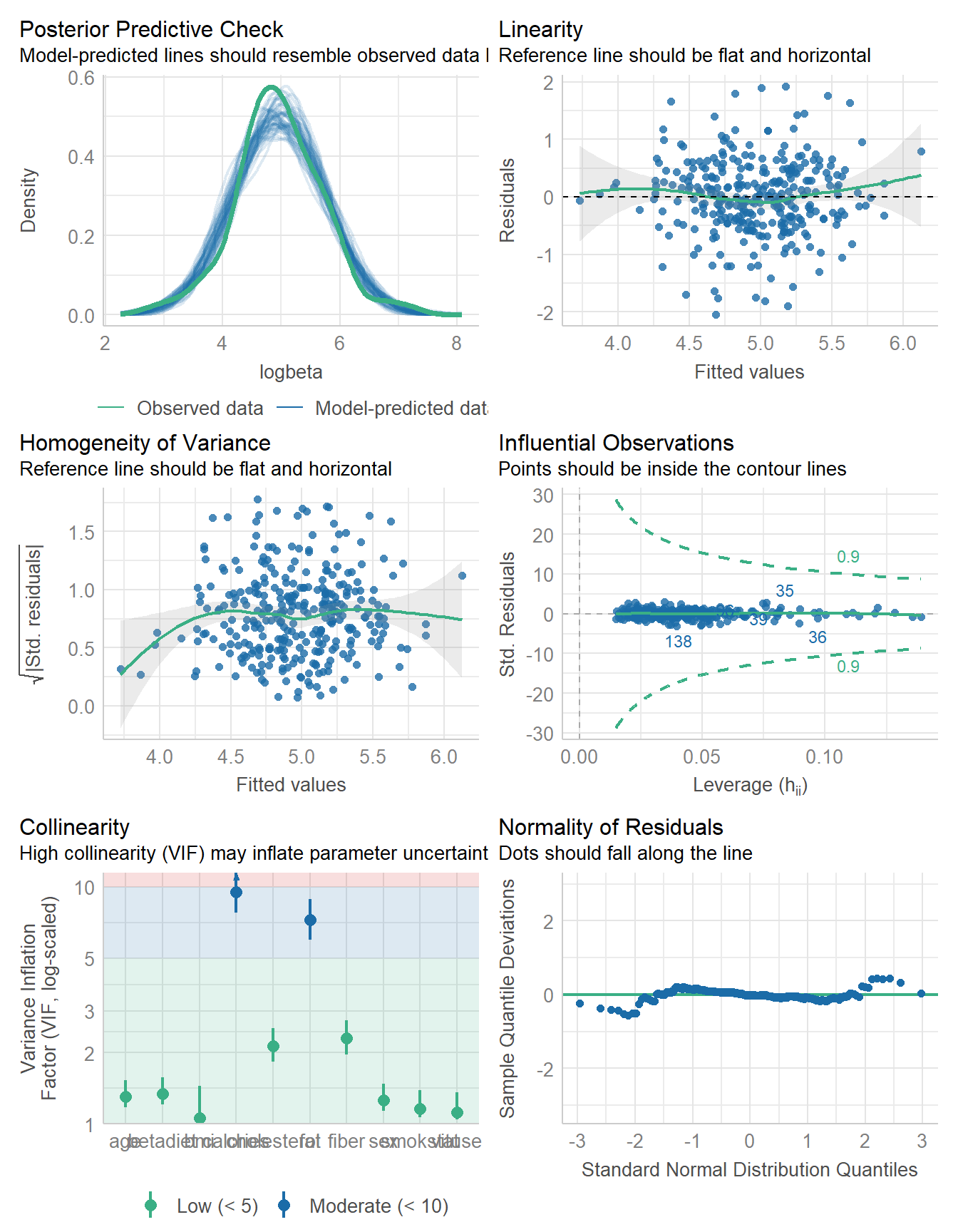
21.4.2 Comparing the Four Models
compare_performance(fit1, fit4, fit8, fit10)# Comparison of Model Performance Indices
Name | Model | AIC (weights) | AICc (weights) | BIC (weights) | R2 | R2 (adj.) | RMSE | Sigma
--------------------------------------------------------------------------------------------------
fit1 | lm | 646.5 (0.059) | 648.1 (0.046) | 702.7 (<.001) | 0.249 | 0.216 | 0.648 | 0.663
fit4 | lm | 647.7 (0.033) | 648.0 (0.047) | 673.9 (0.998) | 0.206 | 0.193 | 0.666 | 0.672
fit8 | lm | 641.3 (0.775) | 642.4 (0.794) | 686.3 (0.002) | 0.247 | 0.222 | 0.649 | 0.660
fit10 | lm | 644.8 (0.134) | 646.2 (0.114) | 697.3 (<.001) | 0.248 | 0.218 | 0.648 | 0.662plot(compare_performance(fit1, fit4, fit8, fit10))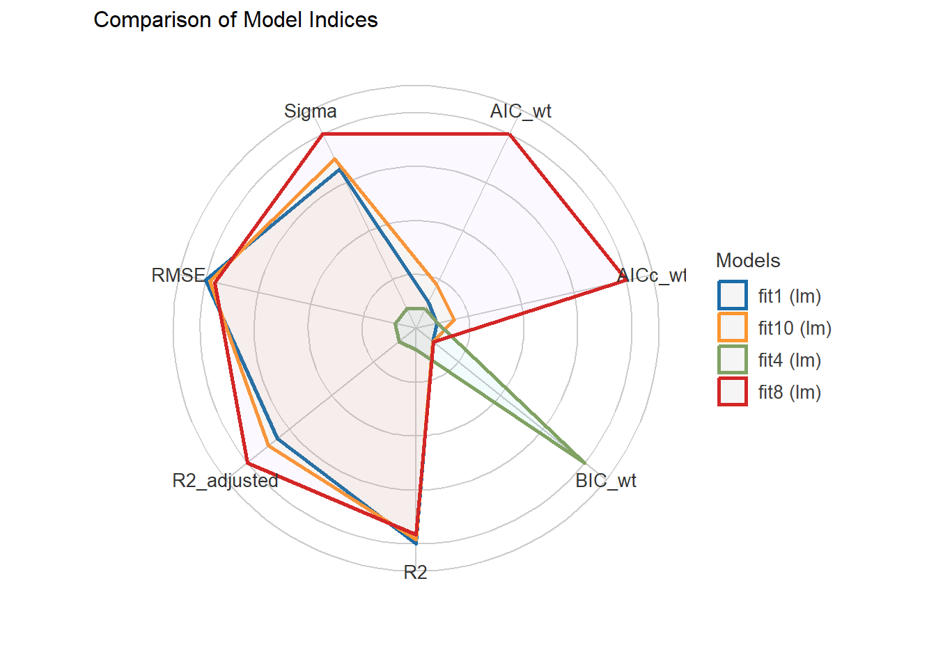
Within our sample, it looks like fit8 is the strongest of these models.
How about its cross-validation performance?
set.seed(431)
performance_accuracy(fit10, method = "cv", k = 5)
# Accuracy of Model Predictions
Accuracy (95% CI): 42.65% [32.47%, 52.20%]
Method: Correlation between observed and predictedset.seed(431)
performance_cv(fit10)# Cross-validation performance (30% holdout method)
MSE | RMSE | R2
-----------------
0.55 | 0.74 | 0.221.4.3 Table of Cross-validated Performance
| Model | Accuracy and 95% CI | MSE\(_{30}\) | RMSE\(_{30}\) | \(R^2_{30}\) |
|---|---|---|---|---|
fit1 |
.4242 (.3242, .5244) | 0.56 | 0.75 | 0.19 |
fit10 |
.4265 (.3247, .5220) | 0.55 | 0.74 | 0.20 |
fit8 |
.4405 (.3292, .5760) | 0.56 | 0.75 | 0.19 |
fit4 |
.4298 (.3750, .5245) | 0.55 | 0.74 | 0.21 |
It appears that fit8 also performs well in cross-validation, in terms of accuracy. Model fit4 may be a bit better in the measures assessed here using the 30% holdout sample approach. Still, given the strong in-sample performance of fit8, I think I would be inclined to select that model.
21.5 Predicting Plasma Retinol
fit_ret0 <- lm(retplasma ~ age + sex + smokstat + bmi + vituse +
  calories + fat + fiber + alcohol + cholesterol +
  retdiet, data = plasma)

boxCox(fit_ret0)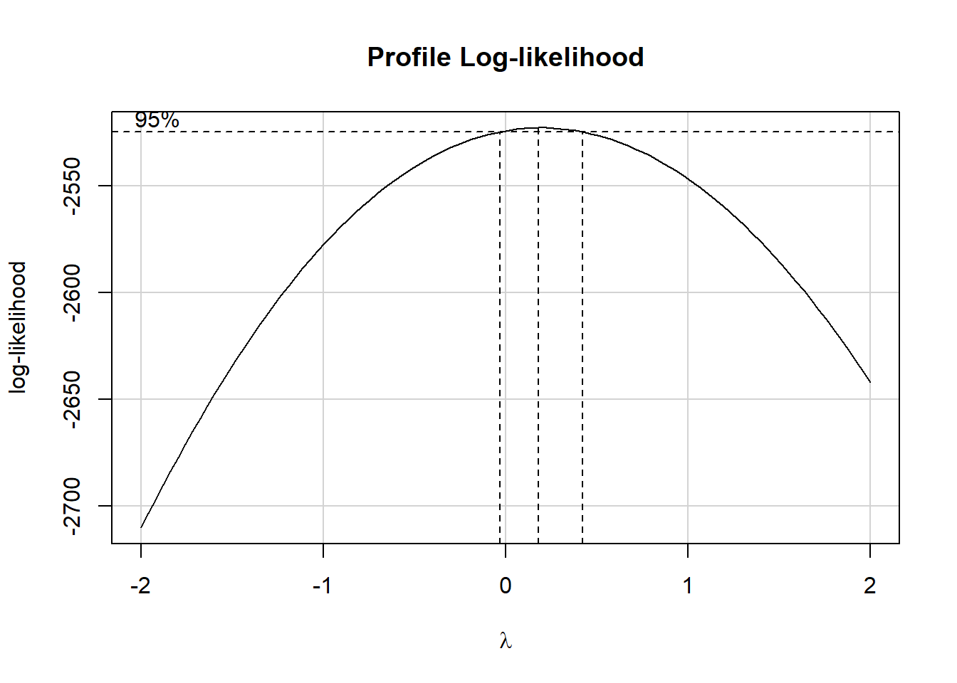
It appears we might want to be working with the logarithm of retplasma as our outcome.
model_parameters(fit_ret1, ci = 0.95)Parameter | Coefficient | SE | 95% CI | t(299) | p
-----------------------------------------------------------------------------
(Intercept) | 6.17 | 0.14 | [ 5.90, 6.44] | 45.37 | < .001
age | 4.98e-03 | 1.43e-03 | [ 0.00, 0.01] | 3.48 | < .001
sex [Male] | 0.06 | 0.06 | [-0.06, 0.18] | 1.00 | 0.316
smokstat [Never] | -0.07 | 0.04 | [-0.15, 0.01] | -1.74 | 0.083
smokstat [Current] | -0.09 | 0.06 | [-0.20, 0.03] | -1.43 | 0.153
bmi | 1.38e-03 | 3.14e-03 | [ 0.00, 0.01] | 0.44 | 0.659
vituse [Not_Often] | 2.27e-03 | 0.05 | [-0.09, 0.09] | 0.05 | 0.962
vituse [Never] | -0.04 | 0.04 | [-0.13, 0.05] | -0.86 | 0.390
calories | 1.51e-04 | 9.81e-05 | [ 0.00, 0.00] | 1.54 | 0.124
fat | -2.93e-03 | 1.54e-03 | [-0.01, 0.00] | -1.90 | 0.058
fiber | -8.58e-03 | 5.04e-03 | [-0.02, 0.00] | -1.70 | 0.090
alcohol | 0.01 | 4.25e-03 | [ 0.00, 0.02] | 2.54 | 0.012
cholesterol | -7.67e-05 | 2.16e-04 | [ 0.00, 0.00] | -0.36 | 0.723
retdiet | 1.99e-06 | 3.57e-05 | [ 0.00, 0.00] | 0.06 | 0.956
Uncertainty intervals (equal-tailed) and p-values (two-tailed) computed
using a Wald t-distribution approximation.model_performance(fit_ret1)# Indices of model performance
AIC | AICc | BIC | R2 | R2 (adj.) | RMSE | Sigma
---------------------------------------------------------------
193.645 | 195.262 | 249.839 | 0.125 | 0.087 | 0.314 | 0.322check_model(fit_ret1)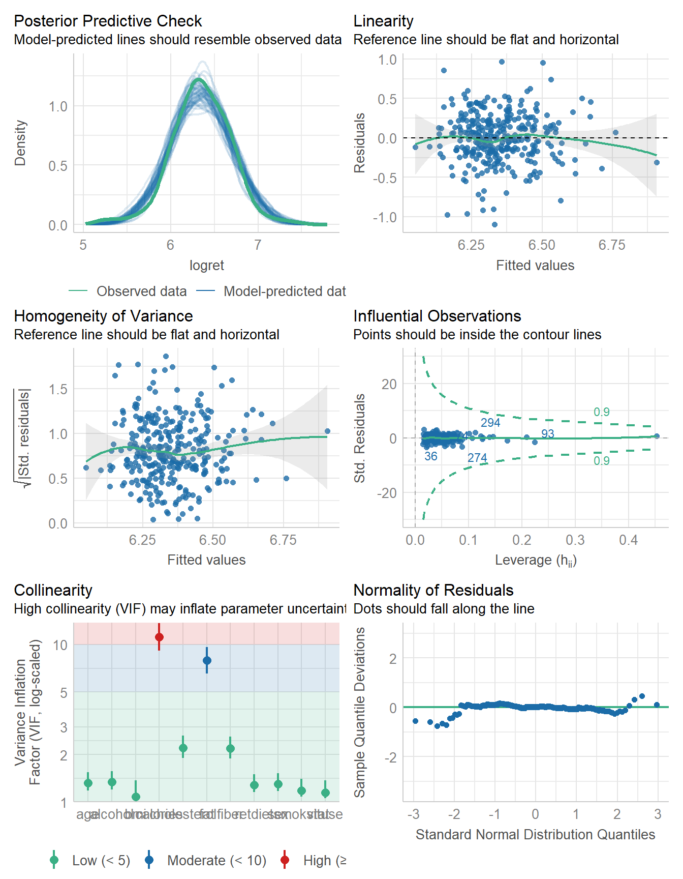
Here, the use of a stepwise approach suggests a 6-predictor subset, including age, smokstat, calories, fat, fiber and alcohol:
fit_ret6 <- select_parameters(fit_ret1)

compare_models(fit_ret1, fit_ret6)
Parameter | fit_ret1 | fit_ret6
----------------------------------------------------------------------
(Intercept) | 6.17 ( 5.90, 6.44) | 6.17 ( 5.97, 6.36)
age | 4.98e-03 ( 0.00, 0.01) | 5.36e-03 ( 0.00, 0.01)
smokstat [Never] | -0.07 (-0.15, 0.01) | -0.07 (-0.15, 0.01)
smokstat [Current] | -0.09 (-0.20, 0.03) | -0.09 (-0.21, 0.02)
calories | 1.51e-04 ( 0.00, 0.00) | 1.65e-04 ( 0.00, 0.00)
fat | -2.93e-03 (-0.01, 0.00) | -3.18e-03 (-0.01, 0.00)
fiber | -8.58e-03 (-0.02, 0.00) | -8.95e-03 (-0.02, 0.00)
alcohol | 0.01 ( 0.00, 0.02) | 0.01 ( 0.00, 0.02)
cholesterol | -7.67e-05 ( 0.00, 0.00) |
bmi | 1.38e-03 ( 0.00, 0.01) |
sex [Male] | 0.06 (-0.06, 0.18) |
vituse [Never] | -0.04 (-0.13, 0.05) |
retdiet | 1.99e-06 ( 0.00, 0.00) |
vituse [Not_Often] | 2.27e-03 (-0.09, 0.09) |
----------------------------------------------------------------------
Observations | 313 | 313I’ll leave for the reader the exercise of evaluating this particular subset, and perhaps developing other potential choices before making additional modeling decisions. One might also consider returning to the data the observation with an unreasonably low betaplasma, since that variable isn’t involved in our prediction of retplasma.
21.6 For More Information
If we run
select_parameters(fit1), that stepwise procedure suggests the 8-predictor subset identified by best subsets, as it turns out.↩︎