11  Association and Regression

11.1 R setup for this chapter

Note

Appendix A lists all R packages used in this book, and also provides R session information. Appendix B describes the 431-Love.R script, and demonstrates its use.

library(GGally)
library(ggpubr)
library(ggstatsplot)
library(glue)
library(janitor)
library(knitr)
library(naniar)
library(patchwork)
library(rstanarm)

library(easystats)
library(tidyverse)

source("data/Love-431.R")
theme_set(theme_bw())

11.2 Data: US Wooden Roller Coasters

Note

Appendix C provides further guidance on pulling data from other systems into R, while Appendix D gives more information (including download links) for all data sets used in this book.

I was motivated to look at roller coaster¹ data by an older example from the Data and Story Library which also uses the Roller Coaster Database. Specifically, I used this URL to pull data on 110 currently operating (as of late June 2024) wooden roller coasters in the US meeting the following criteria:

• Classification = Roller Coaster
• Design = Sit Down
• Existing
• Location = United States
• Roller Coasters
• Current Status = Operating
• Type = Wood

coasters <- read_csv("data/coasters.csv", show_col_types = FALSE) |>
  janitor::clean_names()

head(coasters)

# A tibble: 6 × 10
  c_id  coaster_n          speed height duration opened park  town  state region
  <chr> <chr>              <dbl>  <dbl>    <dbl>  <dbl> <chr> <chr> <chr> <chr> 
1 C-001 American Eagle      66      127      143   1981 Six … Gurn… Illi… Midwe…
2 C-002 American Thunder    48       82       NA   2008 Six … Eure… Miss… Midwe…
3 C-003 Apocalypse the Ri…  50.1     95      180   2009 Six … Vale… Cali… West  
4 C-004 Arkansas Twister    NA       95       NA   1992 Magi… Hot … Arka… South 
5 C-005 Beast               64.8    110      250   1979 King… Mason Ohio  Midwe…
6 C-006 Big Dipper          NA       NA      100   1958 Camd… Hunt… West… South 

The 10 variables in the data are:

Variable	Description
c_ID	Coaster Identification Code
coaster_N	Name of Coaster
speed	Maximum speed, in miles per hour
height	Maximum height, in feet
duration	Length of ride, in seconds
opened	Year of opening
park	Name of amusement park
town	Name of town where park is located
state	State where park is located
region	Region of the US (4 categories)

11.2.1 Missing Data

The naniar package provides some excellent ways to count missing values in our data.

miss_var_summary(coasters)

# A tibble: 10 × 3
   variable  n_miss pct_miss
   <chr>      <int>    <num>
 1 duration      35    31.8 
 2 speed         17    15.5 
 3 height         9     8.18
 4 c_id           0     0   
 5 coaster_n      0     0   
 6 opened         0     0   
 7 park           0     0   
 8 town           0     0   
 9 state          0     0   
10 region         0     0   

miss_case_table(coasters)

# A tibble: 4 × 3
  n_miss_in_case n_cases pct_cases
           <int>   <int>     <dbl>
1              0      64    58.2  
2              1      32    29.1  
3              2      13    11.8  
4              3       1     0.909

As we’ve done in the past, we’ll restrict ourselves to just the 64 coasters with complete data on all variables. We’ll also set up the ages of the coasters, where age is just 2024 minus the year the coaster opened.

coast_cc <- coasters |>
  mutate(age = 2024 - opened) |>
  drop_na()

coast_cc

# A tibble: 64 × 11
   c_id  coaster_n   speed height duration opened park  town  state region   age
   <chr> <chr>       <dbl>  <dbl>    <dbl>  <dbl> <chr> <chr> <chr> <chr>  <dbl>
 1 C-001 American E…  66      127      143   1981 Six … Gurn… Illi… Midwe…    43
 2 C-003 Apocalypse…  50.1     95      180   2009 Six … Vale… Cali… West      15
 3 C-005 Beast        64.8    110      250   1979 King… Mason Ohio  Midwe…    45
 4 C-007 Blue Streak  40       78      105   1964 Ceda… Sand… Ohio  Midwe…    60
 5 C-013 Classic Co…  50       55      105   1935 Wash… Puya… Wash… West      89
 6 C-014 Coastersau…  32       40       50   2004 Lego… Wint… Flor… South     20
 7 C-015 Comet        50       84      105   1946 Hers… Hers… Penn… North…    78
 8 C-016 Comet        55       95      120   1994 Six … Quee… New … North…    30
 9 C-017 Comet        25       37       84   1951 Wald… Erie  Penn… North…    73
10 C-019 Cyclone      60       75      110   1927 Luna… Broo… New … North…    97
# ℹ 54 more rows

11.3 Exploratory Data Analysis

11.3.1 Visualizations

Although we’re primarily interested in associations between variables, let’s look briefly at the sample distributions for the four variables of interest.

p1 <- ggplot(coast_cc, aes(x = speed)) +
  geom_histogram(bins = 8, fill = "red", col = "yellow") +
  labs(title = "Speed in MPH")

p2 <- ggplot(coast_cc, aes(x = height)) +
  geom_histogram(bins = 8, fill = "slateblue", col = "yellow") +
  labs(title = "Height in feet")

p3 <- ggplot(coast_cc, aes(x = duration)) +
  geom_histogram(bins = 8, fill = "magenta", col = "yellow") +
  labs(title = "Duration in seconds")

p4 <- ggplot(coast_cc, aes(x = age)) +
  geom_histogram(bins = 8, fill = "seagreen", col = "yellow") +
  labs(title = "Age in years")

(p1 + p2) / (p3 + p4) + 
  plot_annotation(title = "Roller Coaster Data: Quantities",
                  subtitle = "Histograms, n = 64 coasters")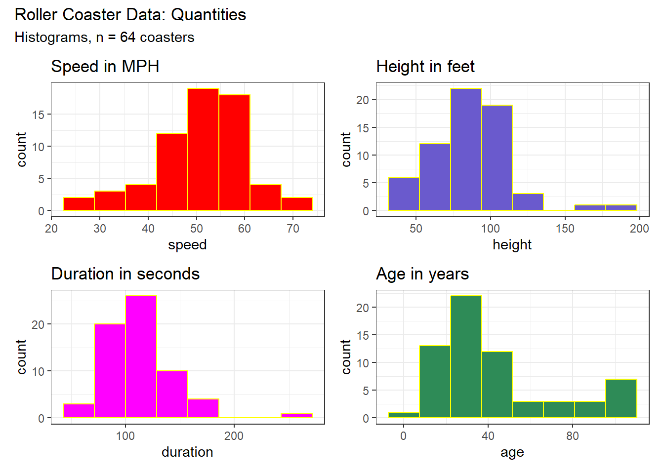

11.3.2 Numeric Summaries

Here are distributional descriptions of our four main variables of interest.

res1 <- coast_cc |> 
  reframe(lovedist(speed)) |>
  mutate(variable = "speed")
res2 <- coast_cc |> 
  reframe(lovedist(height)) |>
  mutate(variable = "height")
res3 <- coast_cc |> 
  reframe(lovedist(duration)) |>
  mutate(variable = "duration")
res4 <- coast_cc |> 
  reframe(lovedist(age)) |>
  mutate(variable = "age")

rbind(res1, res2, res3, res4) |>
  relocate(variable) |>
  kable(digits = 2)

variable	n	miss	mean	sd	med	mad	min	q25	q75	max
speed	64	0	50.76	9.06	51.15	7.19	25	45.75	56.00	70
height	64	0	86.20	26.19	85.00	22.24	35	70.75	100.00	181
duration	64	0	112.67	31.71	111.00	28.17	50	90.00	120.00	250
age	64	0	42.72	27.57	33.50	20.76	1	25.00	51.25	104

11.4 height - speed association

First, we’ll consider the association of each coaster’s speed with its height.

11.4.1 Scatterplot with Pearson correlation

Let’s create a plot including both the linear fit (from lm()) and a loess smooth, as well as the Pearson correlation coefficient.

ggplot(coast_cc, aes(x = height, y = speed)) +
  geom_point() +
  geom_smooth(method = "lm", formula = y ~ x, col = "red") +
  geom_smooth(method = "loess", formula = y ~ x, se = FALSE, col = "blue") +
  labs(title = "Association of Speed with Height") +
  annotate("text", x = 150, y = 40, 
           label = glue("Pearson r = ",
                        round(cor(coast_cc$height, 
                                  coast_cc$speed),3)))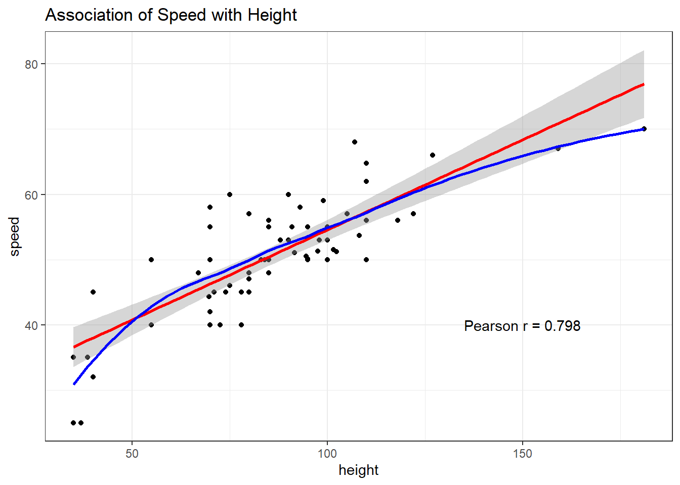

Another way to augment the scatterplot with similar information (other than the loess smooth) follows:

res6 <- cor_test(coast_cc, "height", "speed")

res6

Parameter1 | Parameter2 |    r |       95% CI | t(62) |         p
-----------------------------------------------------------------
height     |      speed | 0.80 | [0.69, 0.87] | 10.43 | < .001***

Observations: 64

plot(res6)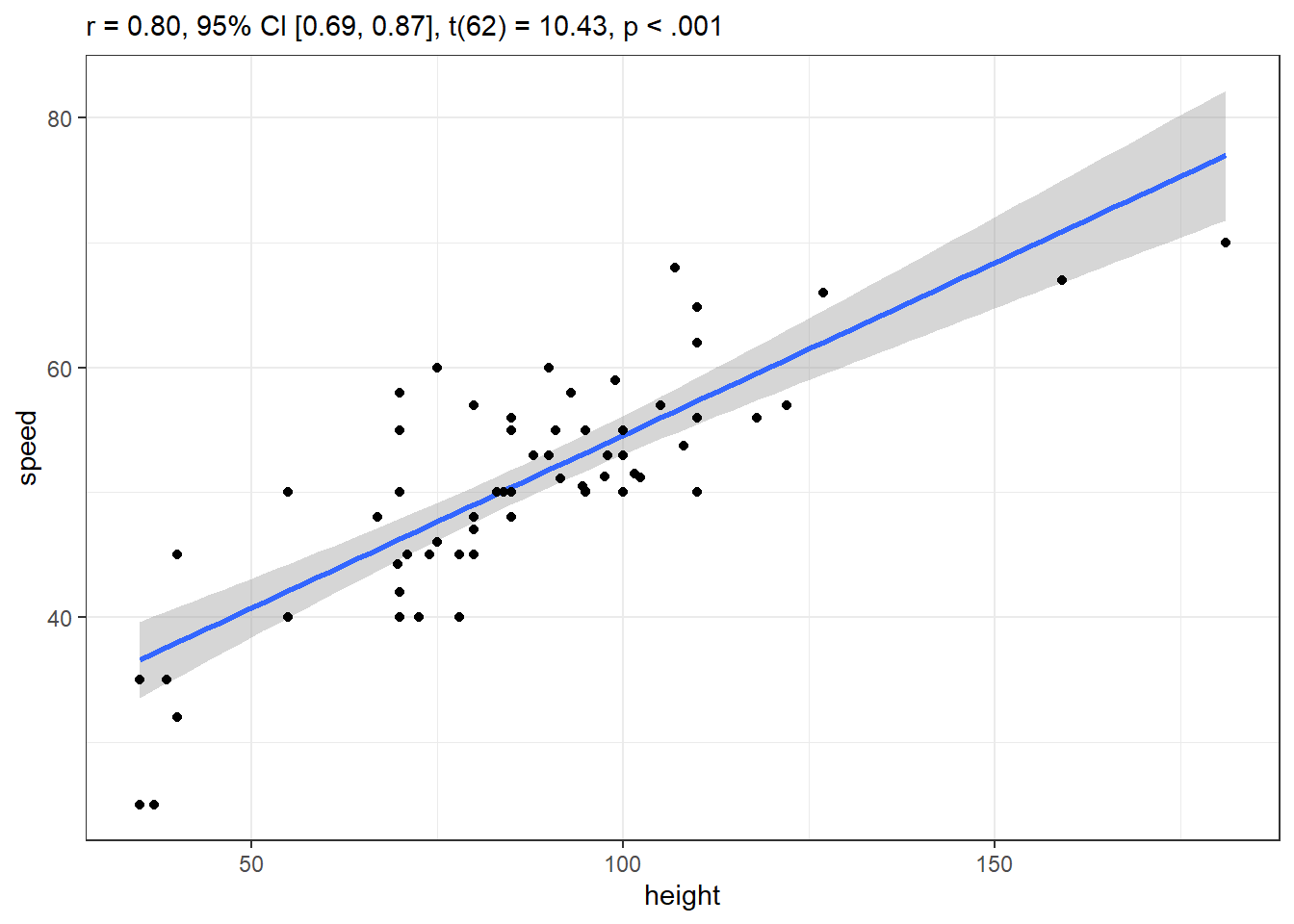

11.4.2 Spearman’s rank correlation

This measure is the Pearson correlation of the rank scores of the two variables. It’s mostly used for assessing whether or not an association is monotone.

cor_test(coast_cc, "height", "speed", method = "spearman")

Parameter1 | Parameter2 |  rho |       95% CI |        S |         p
--------------------------------------------------------------------
height     |      speed | 0.72 | [0.57, 0.82] | 12371.84 | < .001***

Observations: 64

Numerous other measures of association are available. See this description, which is part of easystats’ correlation package.

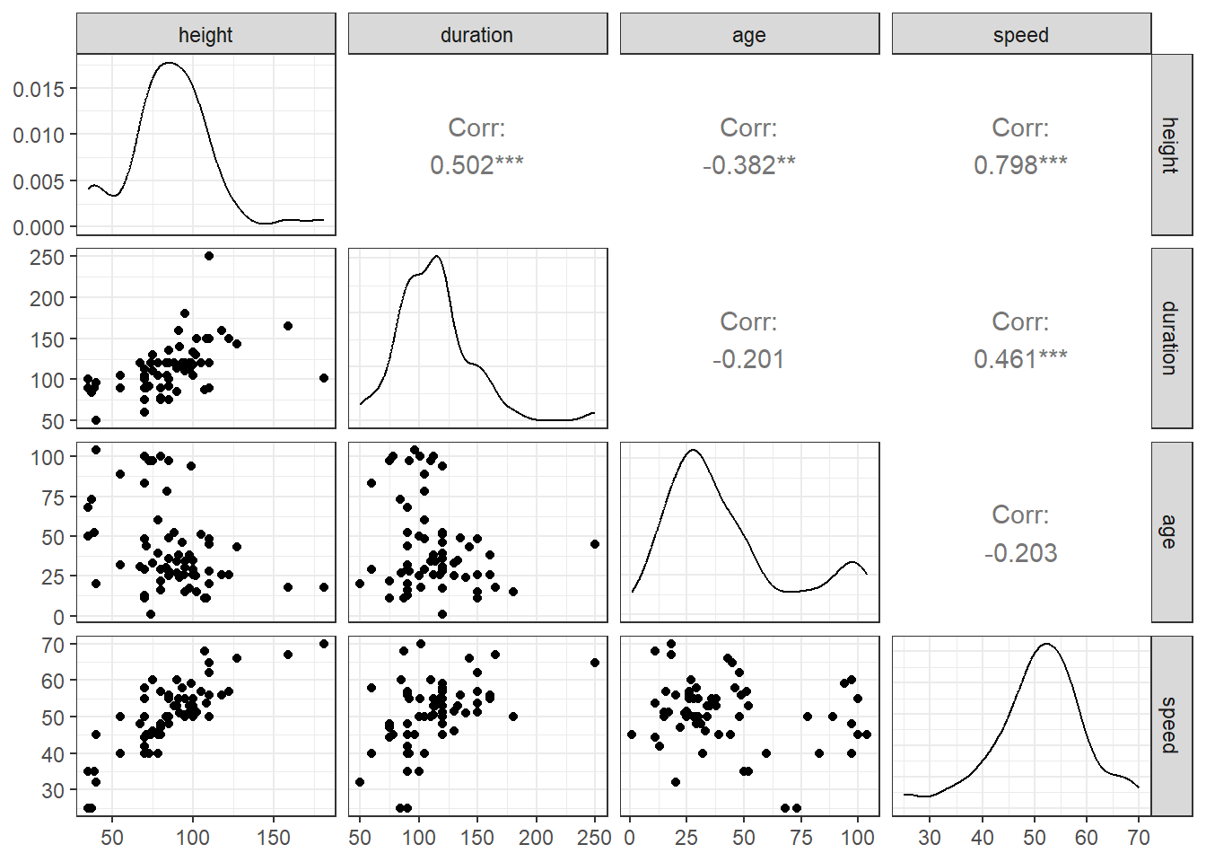
11.5 Scatterplot Matrix

We’ll use the ggpairs function from the GGally package when I want to build a combined matrix of scatterplots and correlation coefficients, as displayed below:

ggpairs(coast_cc |> select(height, duration, age, speed))

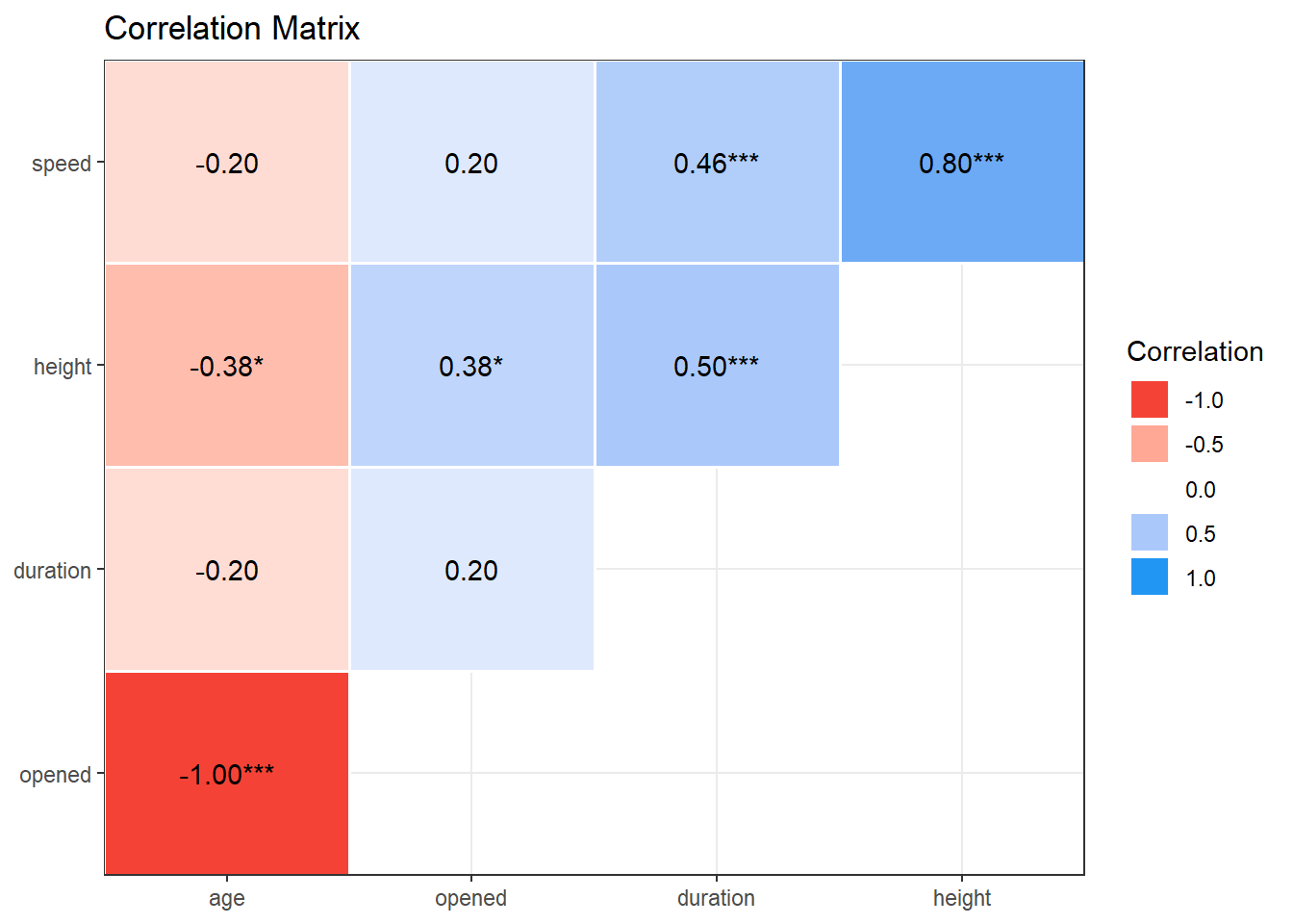
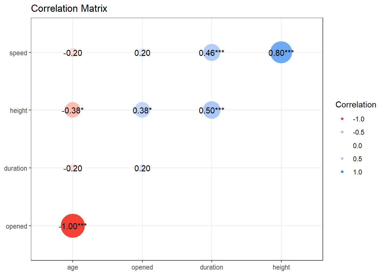
11.6 Correlation Matrix

Behold the complete set of correlation coefficients using the Pearson’s approach for the complete cases in the coasters data.

res_c <- correlation(coast_cc)

res_c

# Correlation Matrix (pearson-method)

Parameter1 | Parameter2 |     r |         95% CI | t(62) |         p
--------------------------------------------------------------------
speed      |     height |  0.80 | [ 0.69,  0.87] | 10.43 | < .001***
speed      |   duration |  0.46 | [ 0.24,  0.63] |  4.09 | < .001***
speed      |     opened |  0.20 | [-0.04,  0.43] |  1.63 | 0.429    
speed      |        age | -0.20 | [-0.43,  0.04] | -1.63 | 0.429    
height     |   duration |  0.50 | [ 0.29,  0.67] |  4.58 | < .001***
height     |     opened |  0.38 | [ 0.15,  0.57] |  3.26 | 0.011*   
height     |        age | -0.38 | [-0.57, -0.15] | -3.26 | 0.011*   
duration   |     opened |  0.20 | [-0.05,  0.43] |  1.62 | 0.429    
duration   |        age | -0.20 | [-0.43,  0.05] | -1.62 | 0.429    
opened     |        age | -1.00 | [-1.00, -1.00] |  -Inf | < .001***

p-value adjustment method: Holm (1979)
Observations: 64

Once we have these results, we can plot them in several ways, in addition to the scatterplot matrix we’ve seen. These include:

plot(summary(res_c))

and

plot(summary(res_c), show_data = "points")

11.6.1 Using a different measure

We can also obtain a correlation matrix using Spearman’s rank correlation, as follows:

res8 <- correlation(coast_cc, method = "spearman")

res8

# Correlation Matrix (spearman-method)

Parameter1 | Parameter2 |   rho |         95% CI |        S |         p
-----------------------------------------------------------------------
speed      |     height |  0.72 | [ 0.57,  0.82] | 12371.84 | < .001***
speed      |   duration |  0.45 | [ 0.23,  0.63] | 23898.81 | 0.001**  
speed      |     opened |  0.17 | [-0.09,  0.40] | 36461.32 | 0.768    
speed      |        age | -0.17 | [-0.40,  0.09] | 50898.68 | 0.768    
height     |   duration |  0.60 | [ 0.41,  0.74] | 17308.98 | < .001***
height     |     opened |  0.39 | [ 0.15,  0.58] | 26851.92 | 0.010*   
height     |        age | -0.39 | [-0.58, -0.15] | 60508.08 | 0.010*   
duration   |     opened |  0.13 | [-0.12,  0.37] | 37811.21 | 0.768    
duration   |        age | -0.13 | [-0.37,  0.12] | 49548.79 | 0.768    
opened     |        age | -1.00 | [-1.00, -1.00] | 87360.00 | < .001***

p-value adjustment method: Holm (1979)
Observations: 64

11.7 Modeling Speed with Height

Let’s start with a linear model (fit using ordinary least squares) to predict speed using height across our 64 coasters.

11.7.1 Fitting the Model

fit1 <- lm(speed ~ height, data = coast_cc)

11.7.2 Parameter Estimates

model_parameters(fit1, ci = 0.95) |> kable(digits = 2)

Parameter	Coefficient	SE	CI	CI_low	CI_high	t	df_error	p
(Intercept)	26.95	2.38	0.95	22.18	31.71	11.31	62	0
height	0.28	0.03	0.95	0.22	0.33	10.43	62	0

Good ways to interpret these coefficients include:

1. When comparing any two coasters whose heights are one foot apart, we expect a speed that is, on average, 0.28 miles per hour faster, for the taller coaster.
2. Under the fitted model, the average difference in coaster speed between two coasters whose height differs by ten feet is 2.8 MPH.

Note that we multiplied the height difference by ten, so we needed to multiply the average difference by 10, as well, in our second response.

11.7.3 Performance of the Model

How well does our model fit1 perform? Some key summaries (applicable to any of the linear models we’ve fit with ordinary least squares so far in this book, too) are shown below.

model_performance(fit1)

# Indices of model performance

AIC     |    AICc |     BIC |    R2 | R2 (adj.) |  RMSE | Sigma
---------------------------------------------------------------
403.859 | 404.259 | 410.336 | 0.637 |     0.631 | 5.416 | 5.503

While we’ll focus on just a few of these measures in this chapter, specifically R2 and RMSE, here is a description of all of the summaries.

• AIC: Akaike’s Information Criterion
• AICc: Second-order (or small sample) AIC with a correction for small sample sizes
• BIC: Bayesian Information Criterion

AIC, AICc and BIC are used when comparing one or more models for the same outcome. When comparing models fitted by maximum likelihood (like ordinary least squares linear models), the smaller the AIC or BIC, the better the fit. See the R documentation for these information criteria here.

• R2: r-squared value
• R2_adj: adjusted r-squared

The R-squared (\(R^2\)) measure, also called the coefficient of determination, describes how much of the variation in our outcome can be explained using our model (and its predictors.) \(R^2\) falls between 0 and 1, and the closer it is to 1, the better the model fits our data. In a simple linear regression model such as we fit here (with one predictor), the \(R^2\) value is also the square of the Pearson correlation coefficient. Note also that in discussing ANOVA previously, we called the \(R^2\) value \(\eta^2\).

An adjusted R-squared measure, is an index (so it’s no longer a proportion of anything) used to compare different models (usually using different sets of predictors) that are fit to predict the same outcome. While adjusted \(R^2\) usually falls between 0 and 1, it can also be negative, and its formula takes into account both the number of observations available and the number of predictors in the model. The idea is to reduce the temptation to overfit the data, by penalizing the \(R^2\) value a little for each predictor. The adjusted \(R^2\) measure is always no larger than \(R^2\). See the documentation for these measures in the performance package (part of easystats.)

• RMSE: root mean squared error
• SIGMA: residual standard deviation, see insight::get_sigma()

The RMSE is the square root of the variance of the residuals and indicates the absolute fit of the model to the data (difference between observed data to model’s predicted values). It can be interpreted as the standard deviation of the unexplained variance, and is in the same units as the response variable. Lower values indicate better model fit. (Source).

Linear models assume that their residuals are drawn from a Normal distribution with mean 0 and standard deviation equal to sigma (\(\sigma\)). The residual standard deviation sigma indicates the accuracy for a model to predict our outcome. \(\sigma\) also indicates that the predicted outcome will be within \(\pm 1 \sigma\) units of the observed outcome for approximately 68% of the data points, for example. See the discussion of sigma here.

11.8 Checking a Linear Model

The main assumptions of any linear model are:

• linearity: we assume that the outcome is linearly related to our predictor
• constant variance (homoscedasticity): we assume that the variation of our outcome is about the same regardless of the value of our predictor
• normal distribution: we assume that the errors around the regression model at any specified values of the x-variables follow an approximately Normal distribution.

11.8.1 Posterior Predictive Checks

Next, we’ll walk through what each of these plots is doing, one at a time.

diagnostic_plots <- plot(check_model(fit1, panel = FALSE))

For confidence bands, please install `qqplotr`.

diagnostic_plots[[1]]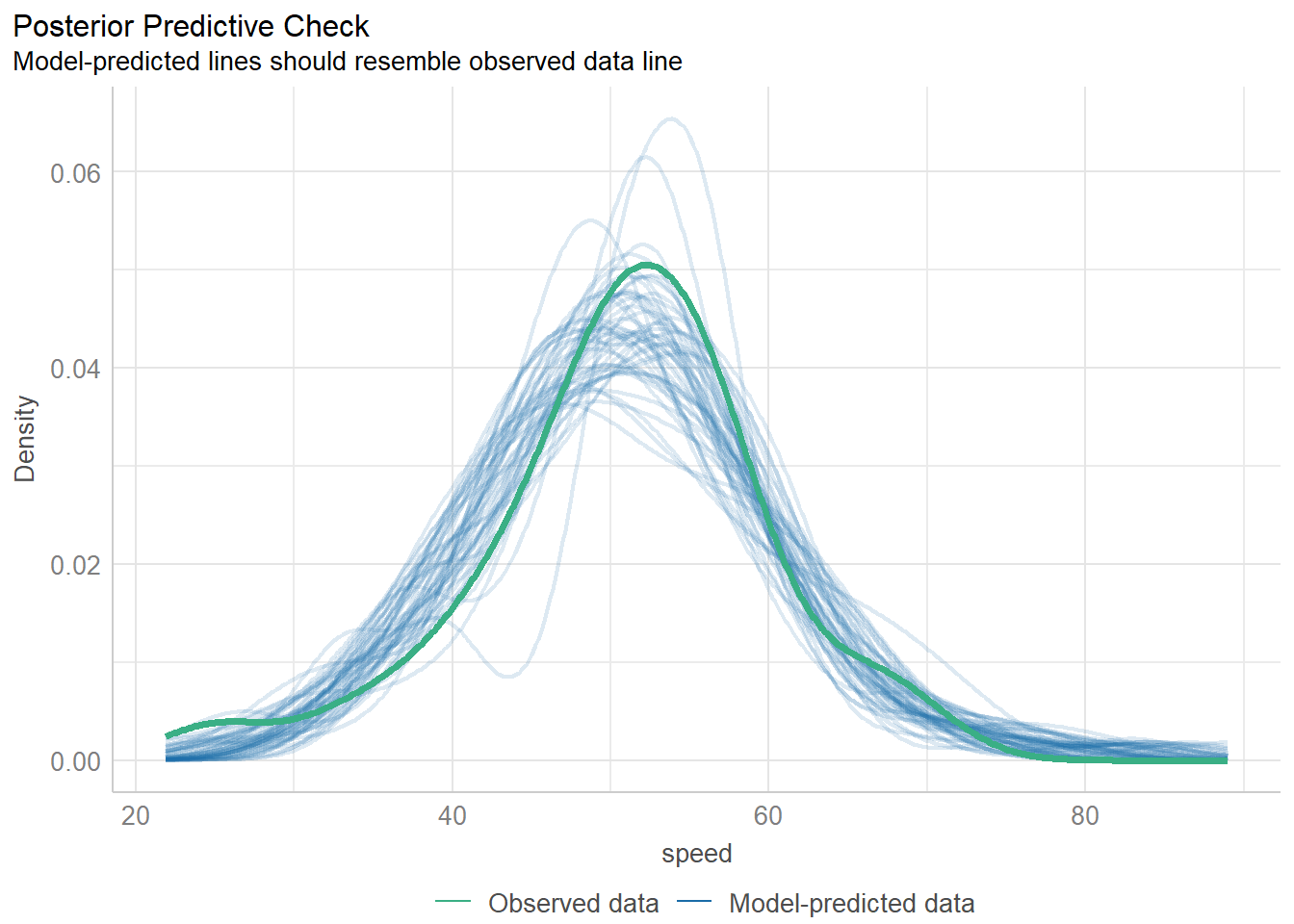

11.8.2 Checking Linearity

diagnostic_plots[[2]]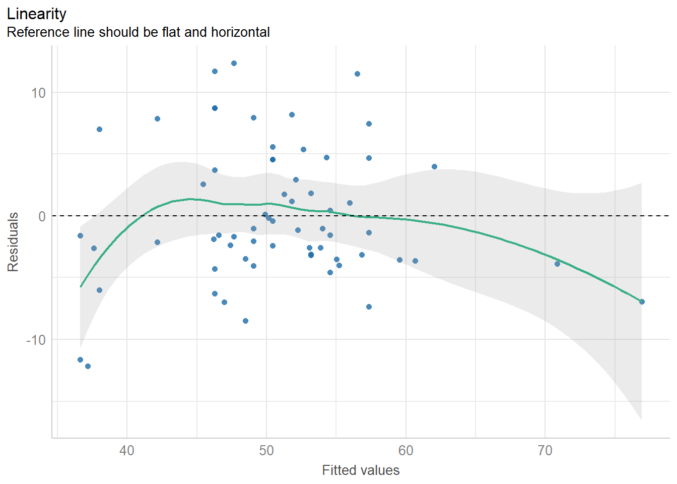

11.8.3 Checking for Homogeneity of Variance

diagnostic_plots[[3]]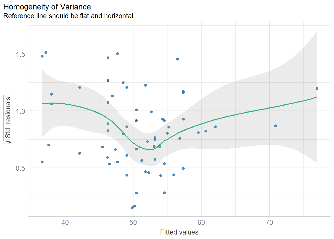

11.8.4 Checking for Influential Observations

diagnostic_plots[[4]]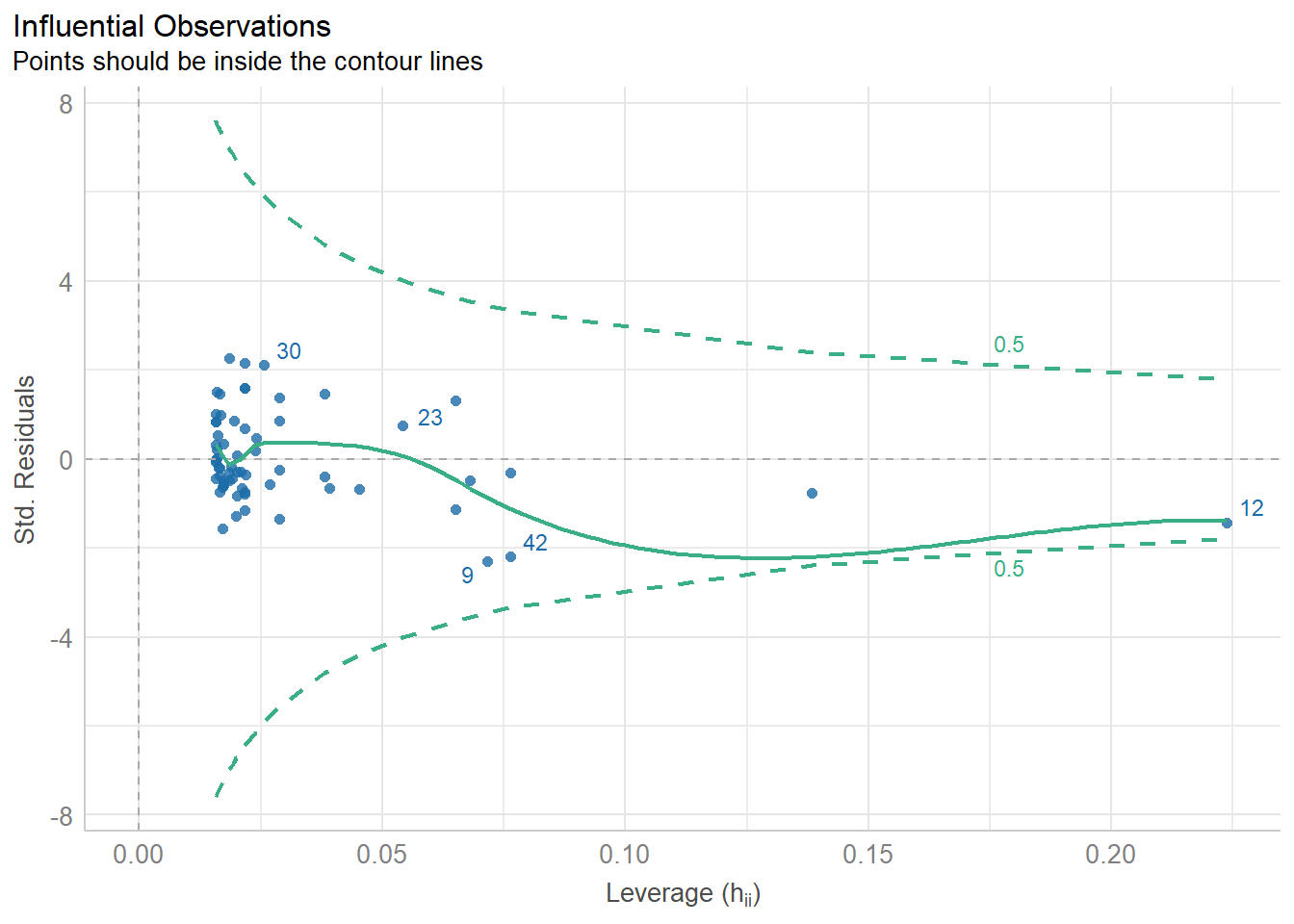

11.8.5 Checking for Normality of Residuals

diagnostic_plots[[5]]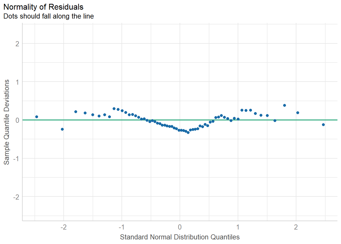

11.8.6 Running All of the Checks

Note

You will want to include

#| fig-height: 9

at the start of the R code chunk where you run check_model() in order to give the plots some vertical space to breathe.

check_model(fit1)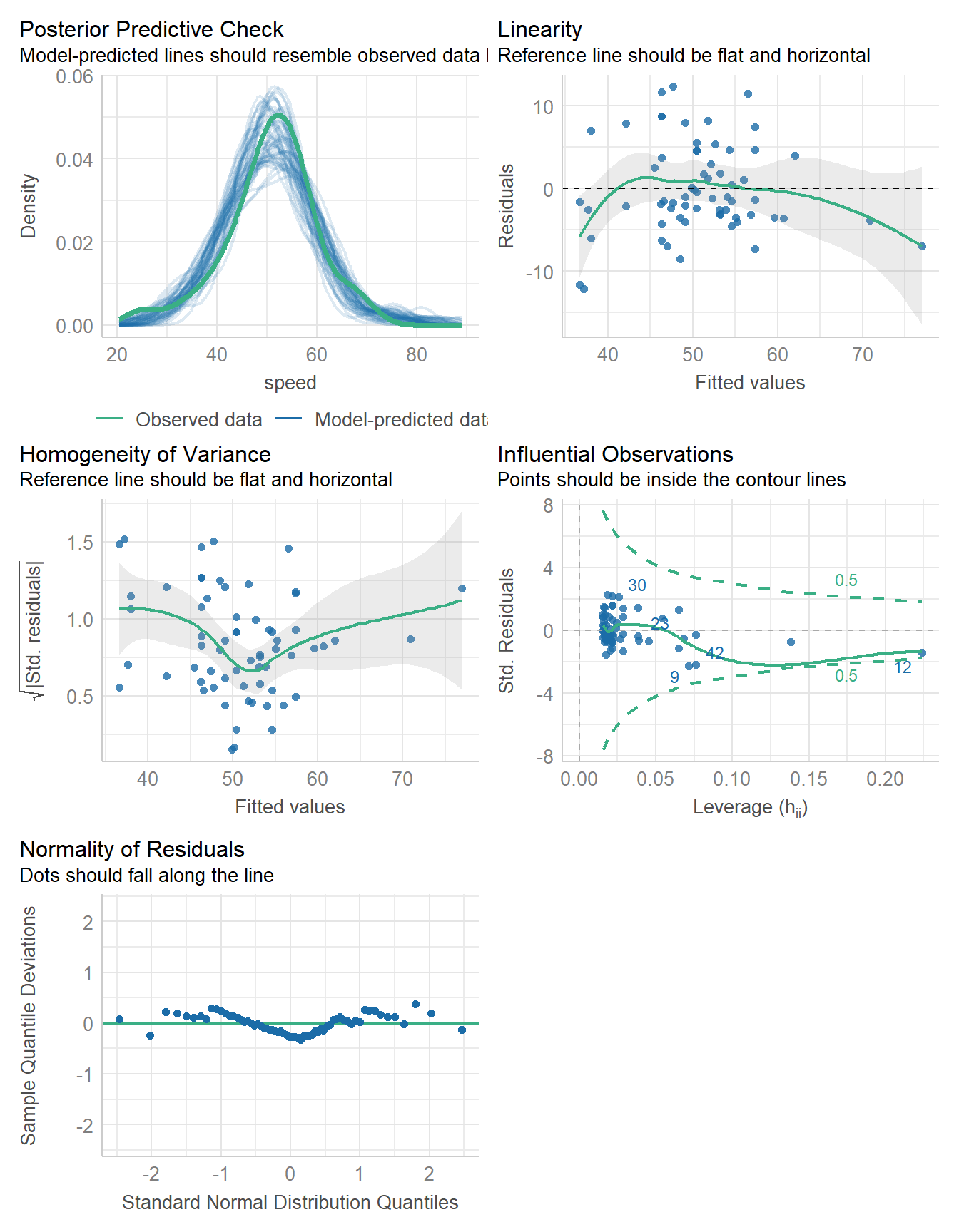

• See the check_model() web page at easystats (performance) for more details.

check_normality(fit1)

OK: residuals appear as normally distributed (p = 0.104).

check_heteroskedasticity(fit1)

OK: Error variance appears to be homoscedastic (p = 0.077).

11.9 Bayesian linear model for Speed with Height

11.9.1 Fitting the model

Here, we fit the Bayesian model, assuming weakly informative priors on the coefficients.

set.seed(431)
fit2 <- stan_glm(speed ~ height, data = coast_cc, refresh = 0)

11.9.2 Parameter Estimates

model_parameters(fit2, ci = 0.95) |> kable(digits = 2)

Parameter	Median	CI	CI_low	CI_high	pd	Rhat	ESS	Prior_Distribution	Prior_Location	Prior_Scale
(Intercept)	26.90	0.95	22.05	31.97	1	1	3770.92	normal	50.76	22.65
height	0.28	0.95	0.22	0.33	1	1	3516.32	normal	0.00	0.87

11.9.3 Performance of the Model

model_performance(fit2)

# Indices of model performance

ELPD     | ELPD_SE |   LOOIC | LOOIC_SE |    WAIC |    R2 | R2 (adj.) |  RMSE | Sigma
-------------------------------------------------------------------------------------
-202.245 |   5.520 | 404.491 |   11.039 | 404.407 | 0.630 |     0.614 | 5.416 | 5.552

11.9.4 Checking the Model

check_model(fit2)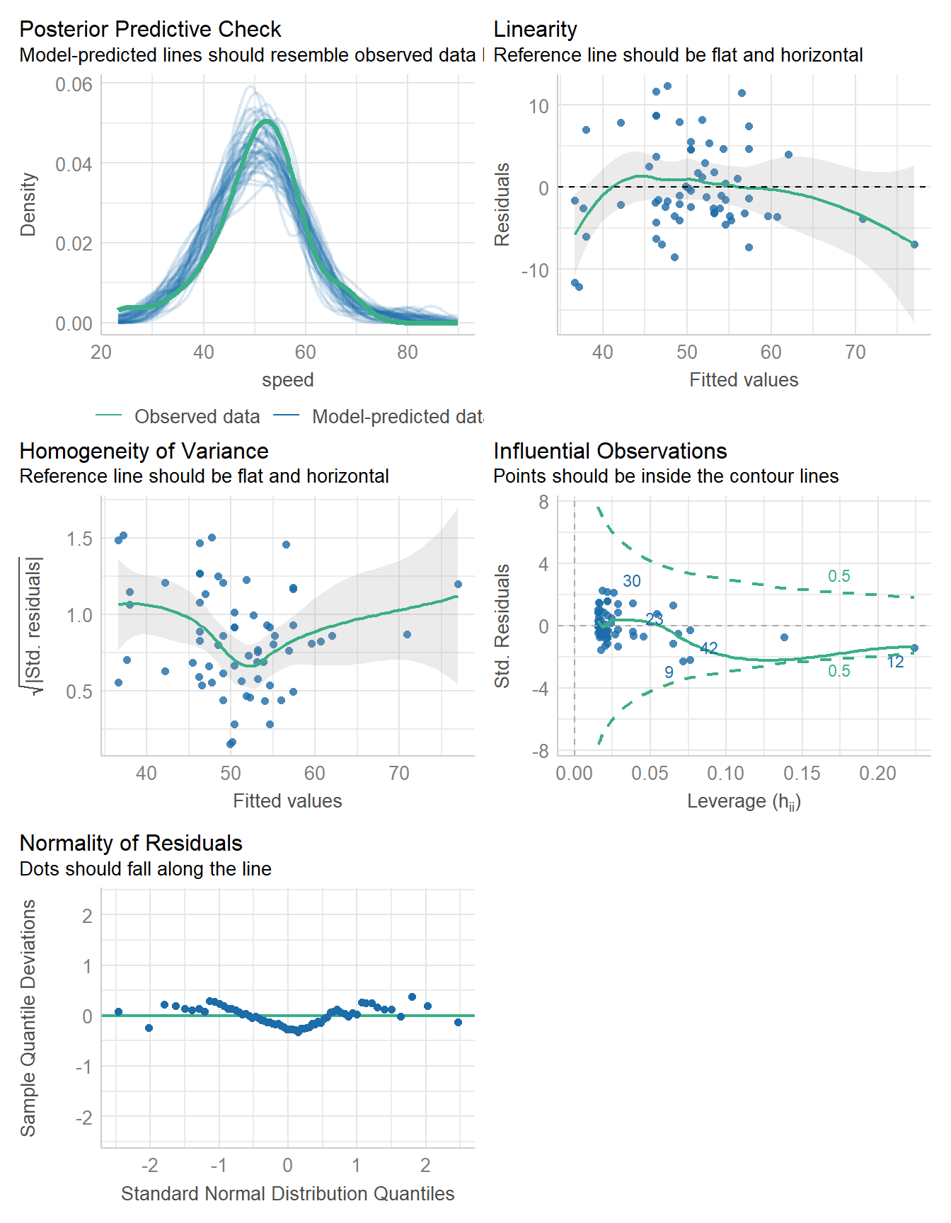

11.10 Predicting Speed with Duration

Next, consider the relationship between duration and speed.

ggplot(coast_cc, aes(x = duration, y = speed)) +
  geom_point() +
  geom_smooth(method = "lm", formula = y ~ x, col = "red") +
  geom_smooth(method = "loess", formula = y ~ x, se = FALSE, col = "blue") +
  labs(title = "Association of Speed with Duration") +
  stat_regline_equation(label.x = 200, label.y = 40) +
  stat_cor(aes(label = after_stat(rr.label)),
    label.x = 200, label.y = 35)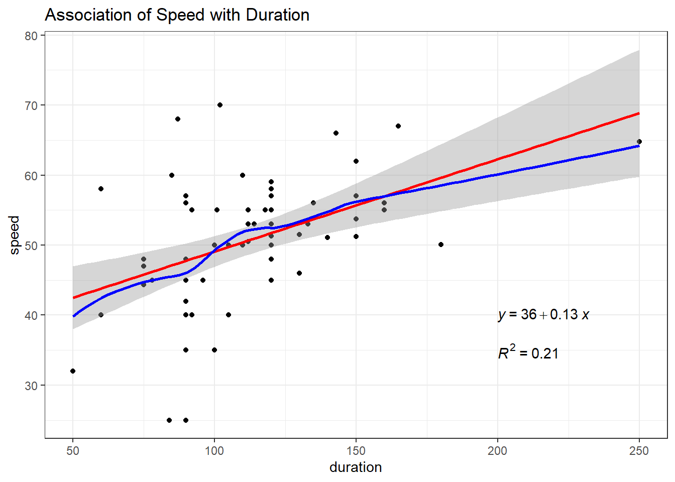

11.10.1 Ordinary Least Squares

fit3 <- lm(speed ~ duration, data = coast_cc)

model_parameters(fit3, ci = 0.95) |> kable(digits = 2)

Parameter	Coefficient	SE	CI	CI_low	CI_high	t	df_error	p
(Intercept)	35.91	3.77	0.95	28.38	43.44	9.53	62	0
duration	0.13	0.03	0.95	0.07	0.20	4.09	62	0

model_performance(fit3) |> kable()

AIC	AICc	BIC	R2	R2_adjusted	RMSE	Sigma
453.4355	453.8355	459.9122	0.2126508	0.1999516	7.97771	8.105361

check_model(fit3)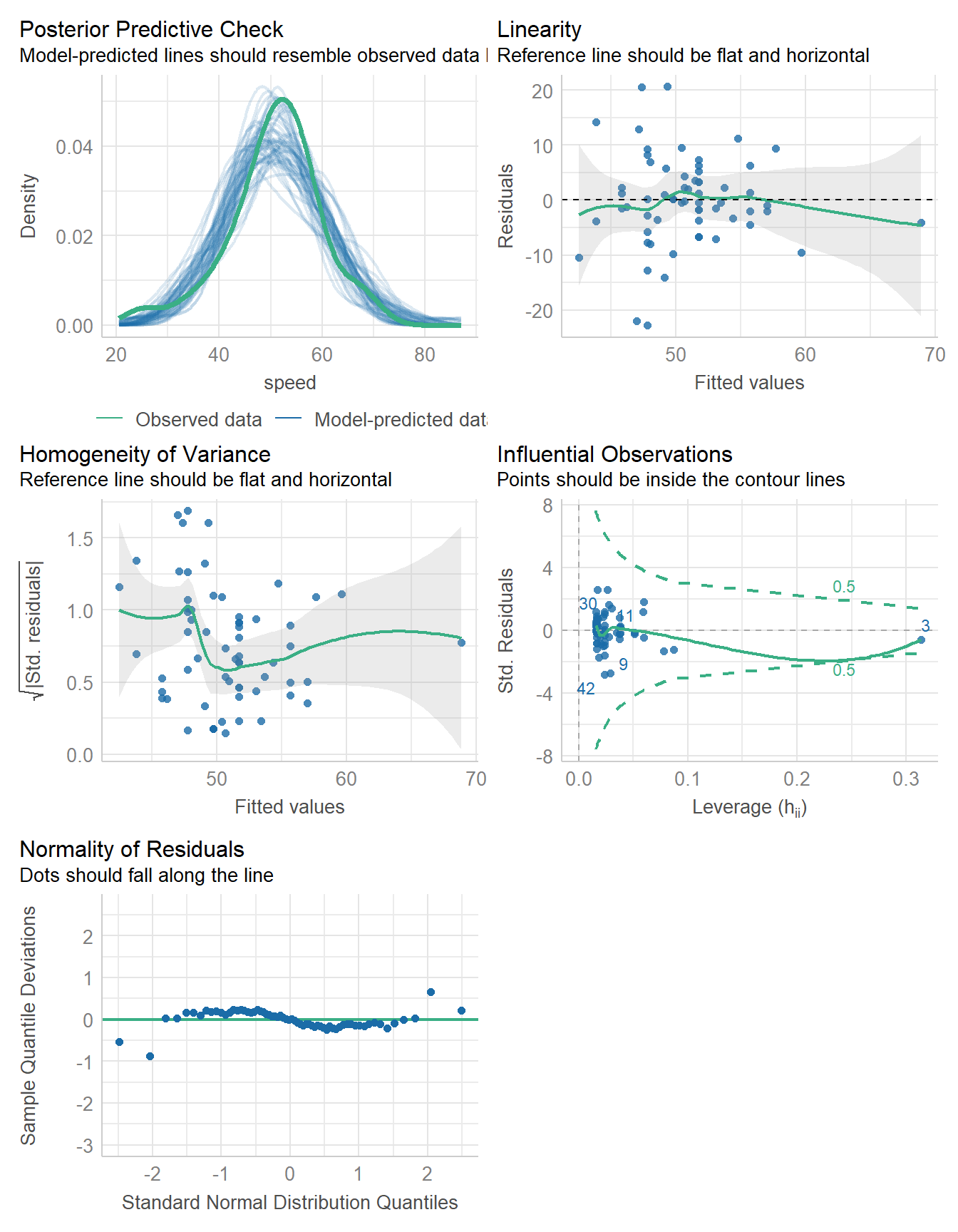

11.10.2 Bayesian linear model fit

set.seed(431)
fit4 <- stan_glm(speed ~ duration, data = coast_cc, refresh = 0)

model_parameters(fit4, ci = 0.95) |> kable(digits = 2)

Parameter	Median	CI	CI_low	CI_high	pd	Rhat	ESS	Prior_Distribution	Prior_Location	Prior_Scale
(Intercept)	35.95	0.95	28.34	43.33	1	1	3722.28	normal	50.76	22.65
duration	0.13	0.95	0.07	0.20	1	1	3704.16	normal	0.00	0.71

model_performance(fit4)

# Indices of model performance

ELPD     | ELPD_SE |   LOOIC | LOOIC_SE |    WAIC |    R2 | R2 (adj.) |  RMSE | Sigma
-------------------------------------------------------------------------------------
-227.090 |   7.486 | 454.181 |   14.972 | 454.127 | 0.209 |     0.180 | 7.978 | 8.168

check_model(fit4)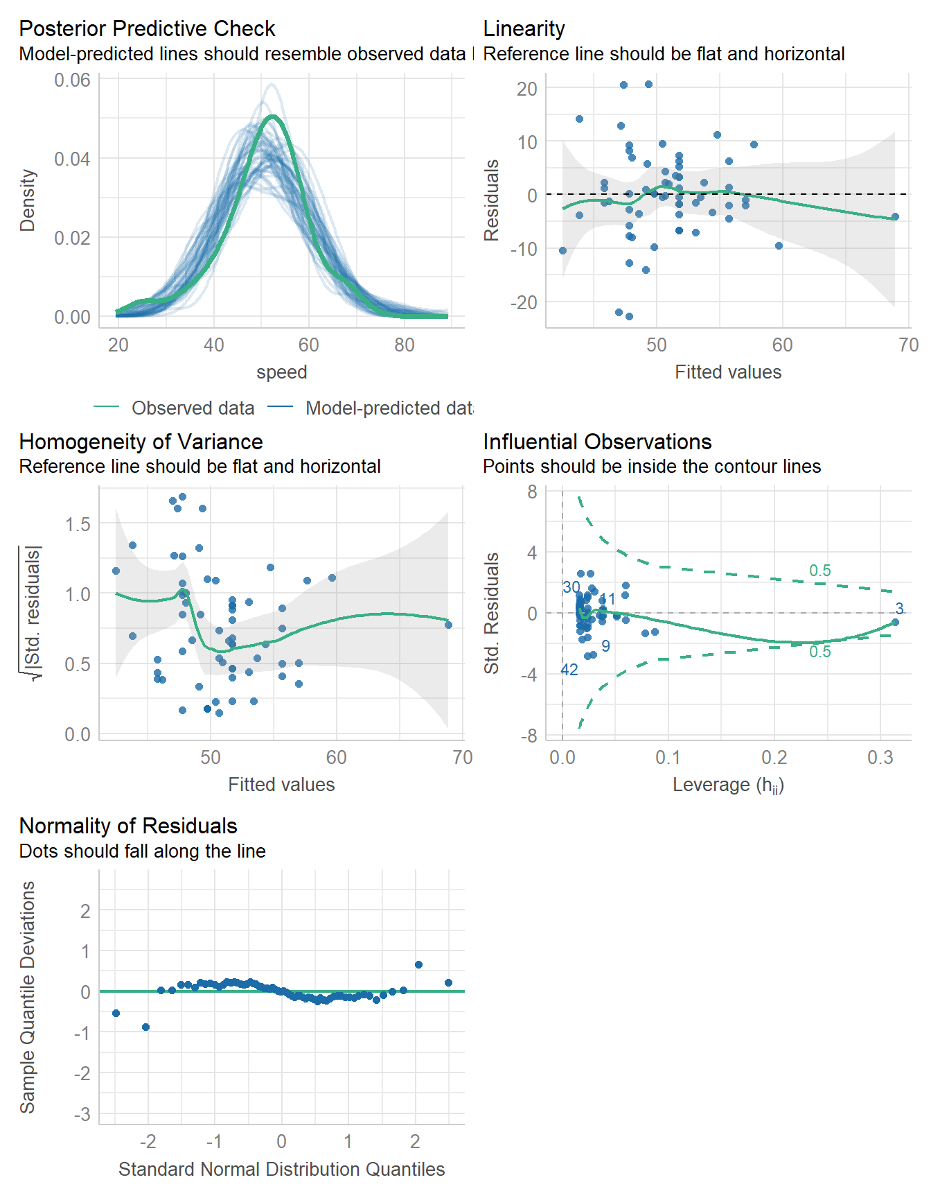

11.11 Predicting Speed with Age

Finally, are newer coasters faster? Consider the relationship between age and speed.

ggplot(coast_cc, aes(x = age, y = speed)) +
  geom_point() +
  geom_smooth(method = "lm", formula = y ~ x, col = "red") +
  geom_smooth(method = "loess", formula = y ~ x, se = FALSE, col = "blue") +
  labs(title = "Association of Speed with Age") +
  stat_regline_equation(label.x = 65, label.y = 65) +
  stat_cor(aes(label = after_stat(rr.label)),
    label.x = 65, label.y = 60)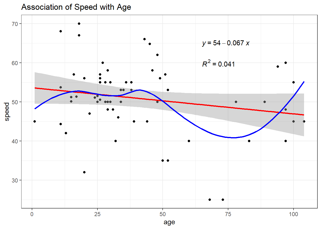

11.11.1 Ordinary Least Squares Fit

fit5 <- lm(speed ~ age, data = coast_cc)

model_parameters(fit5, ci = 0.95) |> kable(digits = 2)

Parameter	Coefficient	SE	CI	CI_low	CI_high	t	df_error	p
(Intercept)	53.61	2.07	0.95	49.47	57.75	25.86	62	0.00
age	-0.07	0.04	0.95	-0.15	0.01	-1.63	62	0.11

model_performance(fit5)

# Indices of model performance

AIC     |    AICc |     BIC |    R2 | R2 (adj.) |  RMSE | Sigma
---------------------------------------------------------------
466.039 | 466.439 | 472.516 | 0.041 |     0.026 | 8.803 | 8.944

check_model(fit5)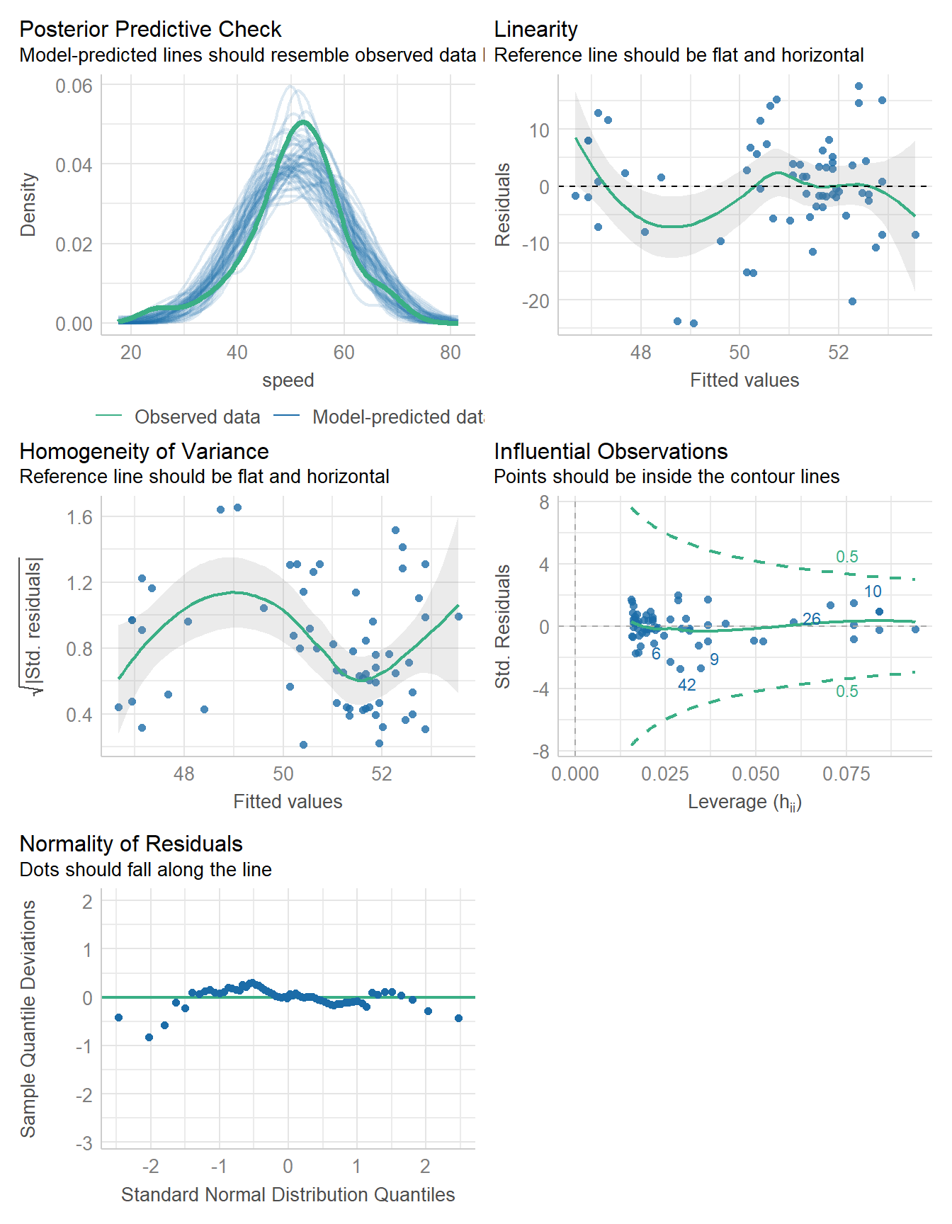

11.11.2 Bayesian linear model fit

set.seed(431)
fit6 <- stan_glm(speed ~ age, data = coast_cc, refresh = 0)

model_parameters(fit6, ci = 0.95) |> kable(digits = 2)

Parameter	Median	CI	CI_low	CI_high	pd	Rhat	ESS	Prior_Distribution	Prior_Location	Prior_Scale
(Intercept)	53.54	0.95	49.57	57.64	1.00	1	3569.63	normal	50.76	22.65
age	-0.07	0.95	-0.15	0.01	0.95	1	3753.96	normal	0.00	0.82

model_performance(fit6)

# Indices of model performance

ELPD     | ELPD_SE |   LOOIC | LOOIC_SE |    WAIC |    R2 | R2 (adj.) |  RMSE | Sigma
-------------------------------------------------------------------------------------
-233.199 |   6.670 | 466.398 |   13.341 | 466.367 | 0.039 |    -0.003 | 8.803 | 8.971

check_model(fit6)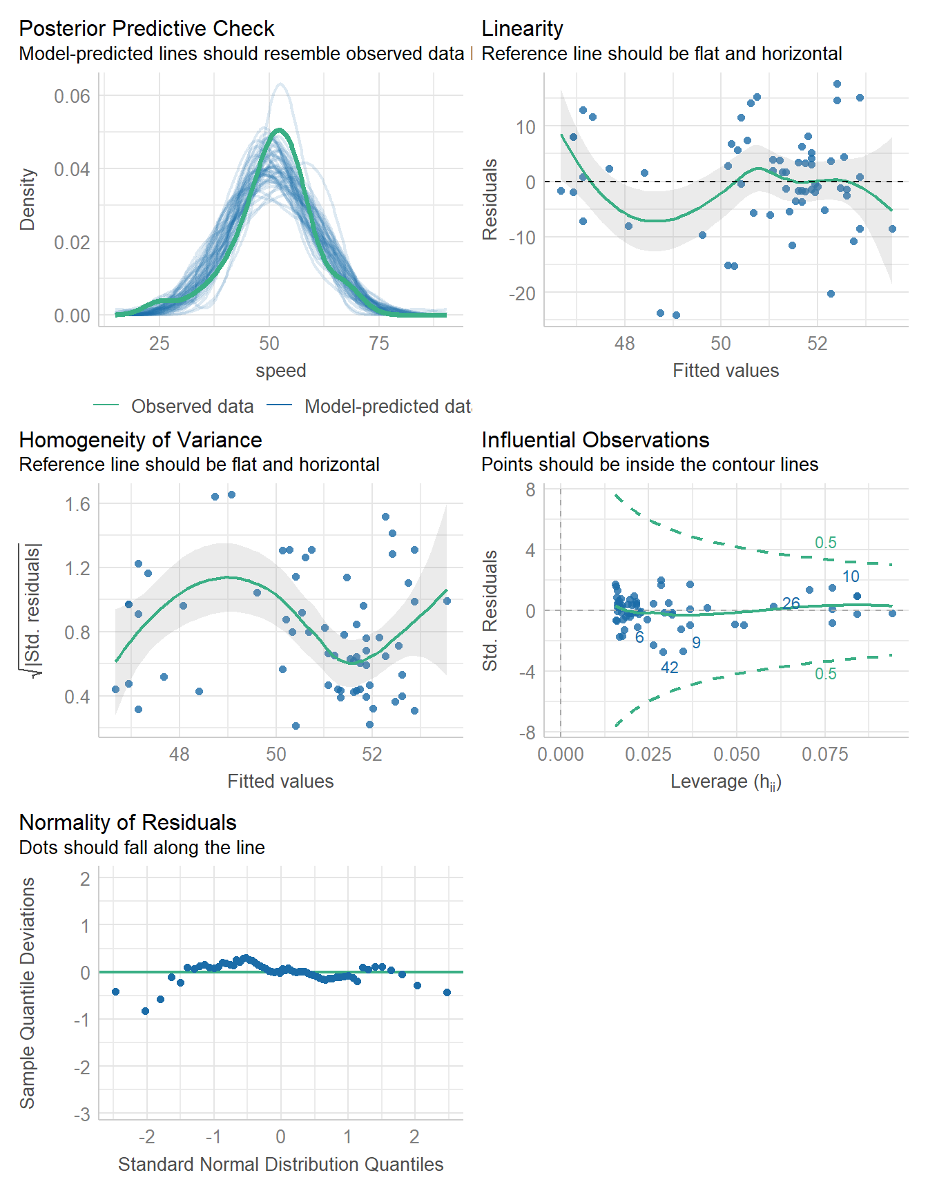

11.12 For More Information

1. Chapter 7 of Çetinkaya-Rundel and Hardin (2024) is about linear regression with a single predictor.
2. This tutorial from the bayestestR package (part of easystats) uses simple linear regression with both lm() and Bayesian approaches.
3. Here is a nice tutorial using R on Simple Linear Regression that addresses some of this chapter’s issues.
4. Wikipedia’s page on Linear regression provides lots of useful details.
5. Plotting Functions for the correlation package
6. Correlation Types

Çetinkaya-Rundel, Mine, and Johanna Hardin. 2024. Introduction to Modern Statistics. Second Edition. OpenIntro Project. https://openintro-ims.netlify.app/.

---

1. My favorite amusement park is Kennywood Park, just outside of Pittsburgh.