9 Comparing Multiple Groups
9.1 R setup for this chapter
Appendix A lists all R packages used in this book, and also provides R session information. Appendix B describes the 431-Love.R script, and demonstrates its use.
9.2 Data from a tab-separated file: Contrast Baths and Carpal Tunnel Syndrome
Appendix C provides further guidance on pulling data from other systems into R, while Appendix D gives more information (including download links) for all data sets used in this book.
Study participants were randomly assigned to one of three treatment group protocols–contrast baths with exercise, contrast baths without exercise, and an exercise-only control treatment group. Study participants were evaluated with hand volumetry, before and after treatment at two different data collection periods-pre- and postoperatively.
The original article is A randomized controlled study of contrast baths on patients with carpal tunnel syndrome by Robert G. Janssen, Deborah A. Schwartz, and Paul F Velleman. I sourced these data from the Data and Story Library.
Data were gathered on 76 participants (59 had complete data on our outcome) before Carpal Tunnel Release surgery. The changes in hand volume (the after treatment volume minus the before treatment volume) are the outcome of interest.
cbaths <- read_tsv("data/cbaths.txt",
                   show_col_types = FALSE) |>
  janitor::clean_names() |>
  mutate(treatment = factor(treatment))

miss_var_summary(cbaths)
# A tibble: 2 × 3
variable n_miss pct_miss
<chr> <int> <num>
1 hand_vol_chg 17 22.4
2 treatment 0 0 ## drop the rows with missing values
cbaths <- cbaths |>
drop_na() cbaths# A tibble: 59 × 2
treatment hand_vol_chg
<fct> <dbl>
1 Bath 10
2 Exercise 0
3 Bath 10
4 Bath 5
5 Exercise 4
6 Bath+Exercise 4
7 Exercise 2
8 Bath -4
9 Bath 8
10 Bath+Exercise 0
# ℹ 49 more rows9.2.1 Summarizing Hand Volume Change by Treatment Group
Our data shows hand volume change (hand_vol_chg) for each subject, as well as which of the three treatments they received. Suppose we want to compare the means of these outcomes across the three treatment groups.
| treatment | n | miss | mean | sd | med | mad | min | q25 | q75 | max |
|---|---|---|---|---|---|---|---|---|---|---|
| Bath | 22 | 0 | 4.55 | 7.76 | 5.5 | 8.15 | -9 | -2.25 | 10.0 | 20 |
| Exercise | 14 | 0 | -1.07 | 5.18 | 0.0 | 2.22 | -12 | -1.00 | 1.5 | 5 |
| Bath+Exercise | 23 | 0 | 8.00 | 7.04 | 7.0 | 10.38 | -2 | 2.00 | 12.5 | 21 |
Our sample sizes are fairly small in each group, so we’ll keep that in mind as we plot the data, thinking about center, spread and shape.
9.2.2 Rain Cloud Plot
ggplot(cbaths, aes(y = treatment, x = hand_vol_chg, fill = treatment)) +
  stat_slab(aes(thickness = after_stat(pdf * n)), scale = 0.7) +
  stat_dotsinterval(side = "bottom", scale = 0.7, slab_linewidth = NA) +
  scale_fill_brewer(palette = "Set2") +
guides(fill = "none") 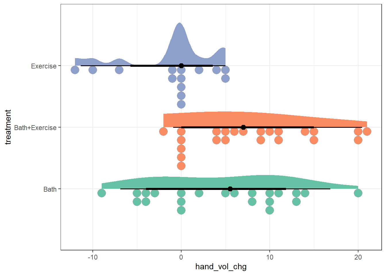
With smaller sample sizes, it’s a bit hard to make strong conclusions about the shape of the data in each group from these plots, or from the boxplots below.
9.2.3 Boxplot and Violin with Means
ggplot(cbaths, aes(x = treatment, y = hand_vol_chg)) +
  geom_violin(aes(fill = treatment)) +
  geom_boxplot(width = 0.15) +
  stat_summary(geom = "point", fun = "mean", col = "red") +
  scale_fill_brewer(palette = "Set2") +
guides(fill = "none") 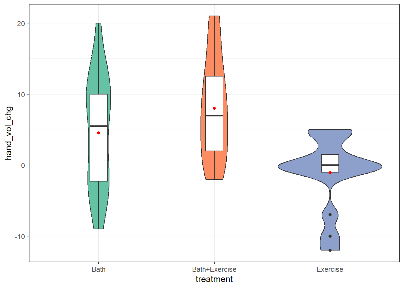
The data in the Bath and Bath+Exercise groups are highly spread out, I think, with the means and medians fairly close to each other. In the Exercise group, we see a few candidate outliers on the low end, and the mean is below even the 25th percentile as a result.
It’s not really clear how willing we should be to assume that the data from each of the samples came from a Normal distribution here, as is often the case with small sample sizes. A linear model does make this assumption when comparing three (or more) group means, but happily is pretty robust to modest violations of that assumption. Let’s run the OLS model and see what we get.
9.3 Comparing Means with a Linear Model
9.3.1 Linear Model Comparing 3 treatment means
Here we build an ordinary least squares (OLS) fit using lm() to predict the outcome based on which of the three treatment groups each subject is in. The predictions made turn out to just be the sample mean of the outcome (hand volume change) in each treatment group. Since we have a small sample size, let’s use a 90% confidence interval here, rather than the default choice of 95%.
fit1 <- lm(hand_vol_chg ~ treatment, data = cbaths)

model_parameters(fit1, ci = 0.90) |> kable(digits = 2)| Parameter | Coefficient | SE | CI | CI_low | CI_high | t | df_error | p |
|---|---|---|---|---|---|---|---|---|
| (Intercept) | 4.55 | 1.48 | 0.9 | 2.07 | 7.02 | 3.07 | 56 | 0.00 |
| treatmentBath+Exercise | 3.45 | 2.07 | 0.9 | -0.01 | 6.92 | 1.67 | 56 | 0.10 |
| treatmentExercise | -5.62 | 2.38 | 0.9 | -9.59 | -1.64 | -2.36 | 56 | 0.02 |
9.3.2 Estimate means at each level from model
means1 <- estimate_means(fit1, ci = 0.90)We selected `by = c("treatment")`.means1Estimated Marginal Means
treatment | Mean | SE | 90% CI
---------------------------------------------
Bath | 4.55 | 1.48 | [ 2.07, 7.02]
Bath+Exercise | 8.00 | 1.45 | [ 5.58, 10.42]
Exercise | -1.07 | 1.86 | [-4.18, 2.03]
Marginal means estimated at treatmentIt looks like, for example, the Bath+Exercise group has a 90% CI which is completely above the Bath group, which is in turn completely above the Exercise group.
Here is a violin plot of each group, on which we’ve included the sample means and the 90% confidence intervals.
plot(visualisation_recipe(means1,
                          show_data = "violin"))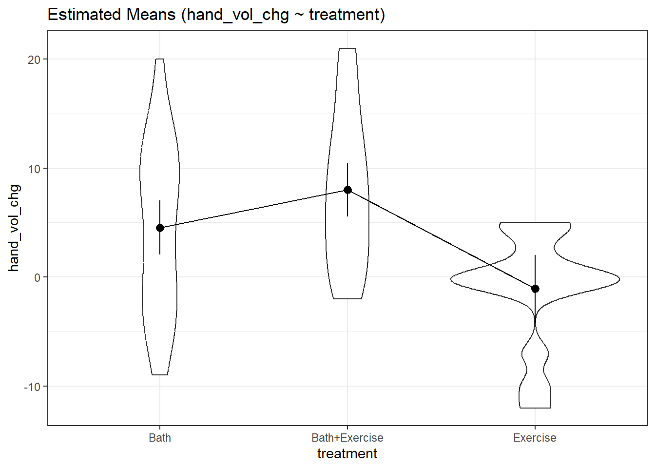
For more on using this approach to visualization when modeling a group of means, you might be interested in this modelbased package vignette.
9.3.3 Assessing Normality
One way to assess whether we have a meaningful problem is to look at some diagnostic plots for our linear model, which we’ll see more of in Chapter 11. But for now, let’s consider a Normal Q-Q plot of the regression residuals for our model fit1 as a way of assessing whether non-Normality in our samples is a serious problem for our fit.
plot(fit1, which = 2)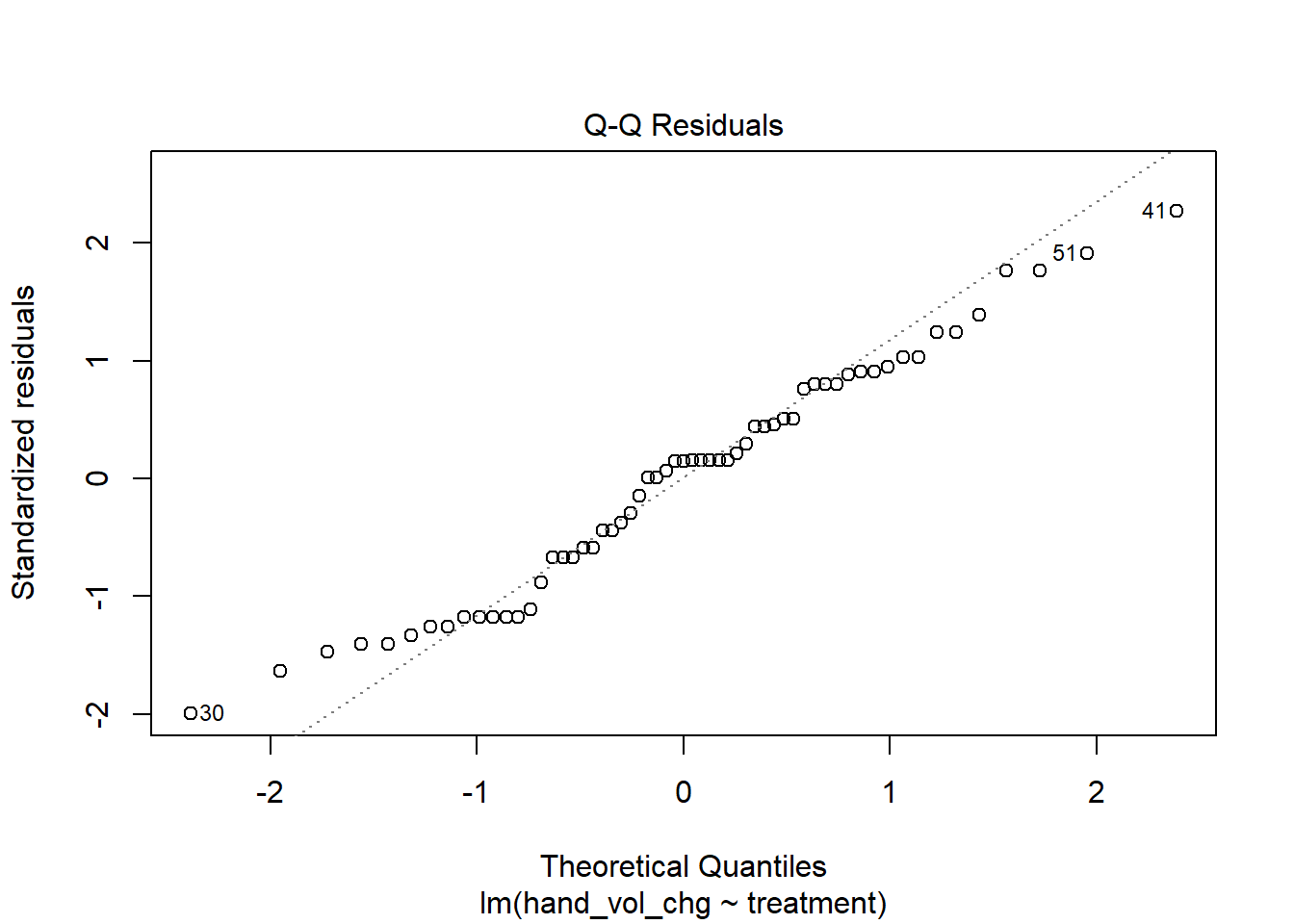
With the possible exception of observation 30 (which may be an outlier), our Normal Q-Q plot of residuals looks pretty good. There’s no evidence of strong violations of the Normality assumption within our fit. So we’ll proceed.
9.3.4 Analysis of Variance Tables
To compare means of two or more independently sampled groups, we can use an analysis of variance (ANOVA) table, which can be generated in at least the following two ways:
anova(fit1)Analysis of Variance Table
Response: hand_vol_chg
Df Sum Sq Mean Sq F value Pr(>F)
treatment 2 716.16 358.08 7.4148 0.001391 **
Residuals 56 2704.38 48.29
---
Signif. codes: 0 '***' 0.001 '**' 0.01 '*' 0.05 '.' 0.1 ' ' 1 Df Sum Sq Mean Sq F value Pr(>F)
treatment 2 716.2 358.1 7.415 0.00139 **
Residuals 56 2704.4 48.3
---
Signif. codes: 0 '***' 0.001 '**' 0.01 '*' 0.05 '.' 0.1 ' ' 1Either one of these ANOVA tables can be used to estimate “eta-squared” (\(\eta^2\)), the proportion of variation explained by the model (which is the sum of squares attributed to the treatment groups - here, 716.16), divided by the total sum of squares (which is 716.16 + 2704.4 = 3420.56.)
We can also obtain an estimate for “eta-squared” (\(\eta^2\)), which is the proportion of variation in our outcome accounted for by the model, i.e. the proportion of variation captured by the means of the treatment groups. Here, the value of \(\eta^2\) is estimated to be 21%.
eta_squared(fit1, ci = 0.90)# Effect Size for ANOVA
Parameter | Eta2 | 90% CI
-------------------------------
treatment | 0.21 | [0.09, 1.00]
- One-sided CIs: upper bound fixed at [1.00].What if we want to directly compare each combination of means (Bath + Exercise to Bath, Exercise to Bath, and Bath + Exercise to Exercise) with 90% confidence intervals? We have two main approaches that we discuss here: Holm’s method (which is a bit superior to the Bonferroni approach in that it’s more powerful) and Tukey’s method (which is appropriate if we pre-planned a set of pairwise comparisons.)
9.3.5 Pairwise Comparisons using Holm method
con1 <- estimate_contrasts(fit1, contrast = "treatment",
                           ci = 0.90, p.adjust = "holm")

con1 |> kable(digits = 2)| Level1 | Level2 | Difference | CI_low | CI_high | SE | df | t | p |
|---|---|---|---|---|---|---|---|---|
| (Bath+Exercise) | Exercise | 9.07 | 3.93 | 14.21 | 2.36 | 56 | 3.85 | 0.00 |
| Bath | (Bath+Exercise) | -3.45 | -7.98 | 1.07 | 2.07 | 56 | -1.67 | 0.10 |
| Bath | Exercise | 5.62 | 0.43 | 10.80 | 2.38 | 56 | 2.36 | 0.04 |
We see that, for example, the comparison of (Bath+Exercise) - Exercise has an estimated mean difference of 9.07, with a 90% confidence interval of (3.93, 14.21). It appears that the combination treatment led to larger hand volume changes, on average.
We can draw similar conclusions about the other two paired comparisons. It’s often helpful to plot these comparisons, and we can do this as follows.
con1_tib <- tibble(con1) |>
  mutate(contr = str_c(Level1, " - ", Level2))

ggplot(con1_tib, aes(x = contr, y = Difference)) +
  geom_point() +
  geom_errorbar(aes(ymin = CI_low, ymax = CI_high)) +
  geom_hline(yintercept = 0, col = "red", lty = "dashed") +
  labs(title = "Holm 90% HSD Intervals for Hand Volume Change",
       x = "Contrast",
       y = "Difference in Hand Volume Change")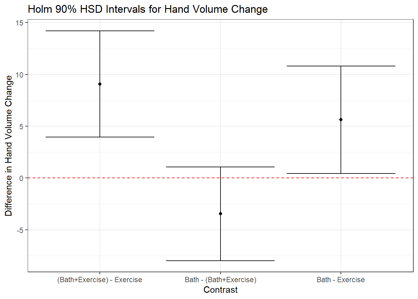
Note that only the Bath - (Bath + Exercise) comparison has a negative point estimate, and it also is the only comparison which has a 90% confidence interval which includes zero. Why might that be interesting?
9.3.6 Pairwise Comparisons using Tukey’s HSD method
Another approach (more powerful than Holm’s approach if we pre-plan our pairwise comparisons) is Tukey’s Honestly Significant Differences method.
con1a <- estimate_contrasts(fit1,
  contrast = "treatment", p_adjust = "tukey", ci = 0.90
)

con1a |> kable(digits = 2)| Level1 | Level2 | Difference | CI_low | CI_high | SE | df | t | p |
|---|---|---|---|---|---|---|---|---|
| (Bath+Exercise) | Exercise | 9.07 | 4.14 | 14.01 | 2.36 | 56 | 3.85 | 0.00 |
| Bath | (Bath+Exercise) | -3.45 | -7.80 | 0.89 | 2.07 | 56 | -1.67 | 0.23 |
| Bath | Exercise | 5.62 | 0.64 | 10.59 | 2.38 | 56 | 2.36 | 0.06 |
Are there important differences in the findings from the Tukey and Holm procedures in this case?
con1a_tib <- tibble(con1a) |>
  mutate(contr = str_c(Level1, " - ", Level2))

ggplot(con1a_tib, aes(y = contr, x = Difference)) +
  geom_point() +
  geom_errorbar(aes(xmin = CI_low, xmax = CI_high)) +
  geom_vline(xintercept = 0, col = "red", lty = "dashed") +
  labs(title = "Tukey 90% HSD Intervals for Hand Volume Change",
       y = "Contrast",
       x = "Difference in Hand Volume Change")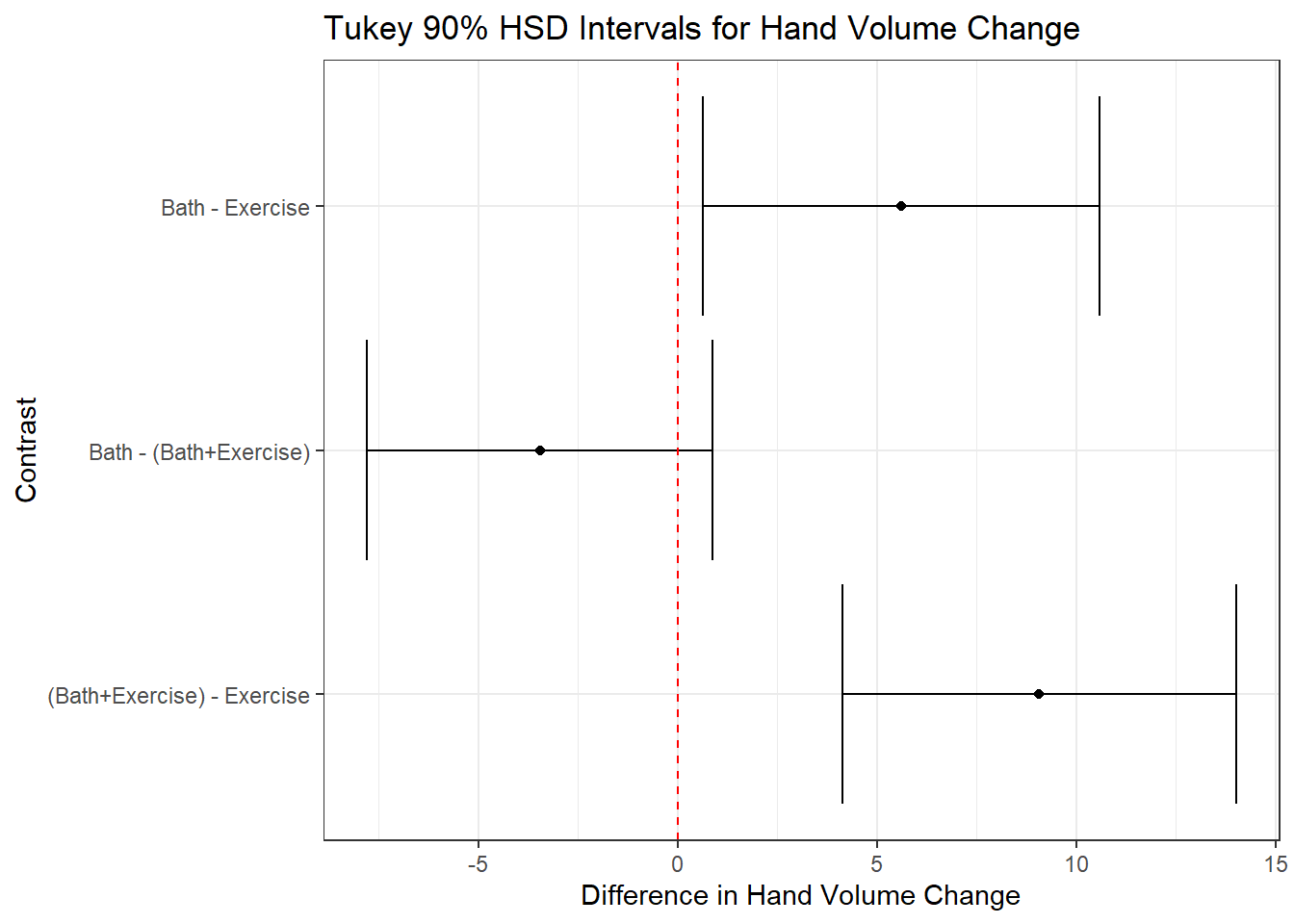
9.4 Bayesian Model comparing 3 means
To fit a Bayesian linear model to compare the mean hand volume changes across our three treatment groups, we can use the following code.
post2 <- describe_posterior(fit2, ci = 0.90)
print_md(post2, digits = 2)| Parameter | Median | 90% CI | pd | ROPE | % in ROPE | Rhat | ESS |
|---|---|---|---|---|---|---|---|
| (Intercept) | 4.58 | [ 2.14, 7.01] | 99.72% | [-0.77, 0.77] | 0% | 1.000 | 3141.00 |
| treatmentBath+Exercise | 3.45 | [ 0.04, 6.87] | 95.12% | [-0.77, 0.77] | 7.82% | 1.000 | 2951.00 |
| treatmentExercise | -5.70 | [-9.72, -1.74] | 98.95% | [-0.77, 0.77] | 0% | 0.999 | 3201.00 |
We see that the model selects the Bath only group as its baseline, with an estimated mean (based on the median of the posterior distribution) of 4.58, with 90% credible interval (2.14, 7.01).
The difference between Bath only and Bath+Exercise is estimated to be 3.45 (with higher values for the Bath+Exercise group) with 90% credible interval (0.04, 6.87).
The difference between Bath only and Exercise only is estimated to be 5.70 (with higher values for the Bath group) with 90% credible interval (1.74, 9.72).
Here is the plot of these three effects, showing the 90% credible intervals.
plot(fit2,
  plotfun = "areas", prob = 0.90,
  pars = c("(Intercept)", "treatmentBath+Exercise",
           "treatmentExercise"))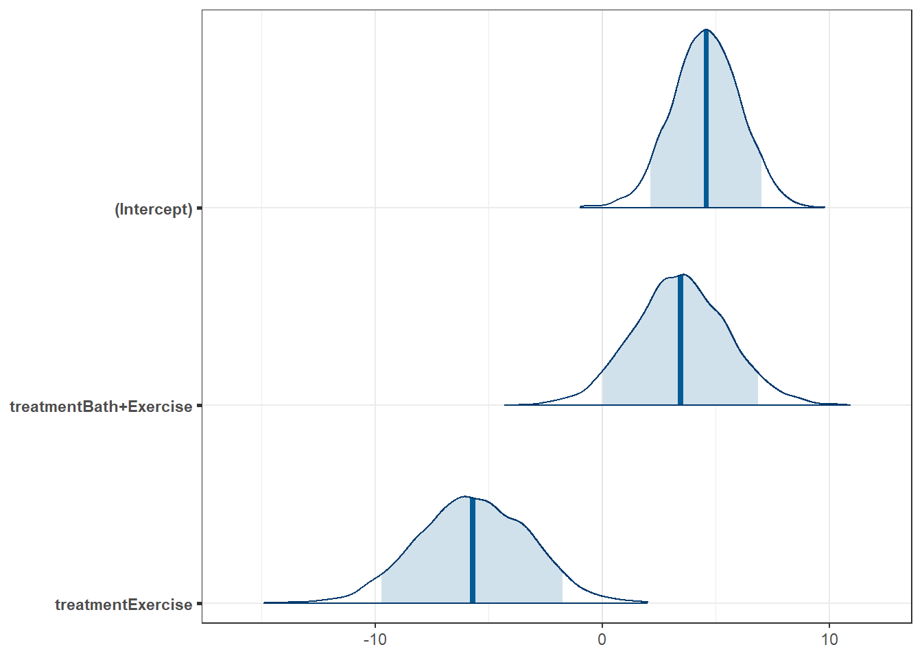
fit2 |> model_parameters(ci = 0.90) |> kable(digits = 2)| Parameter | Median | CI | CI_low | CI_high | pd | Rhat | ESS | Prior_Distribution | Prior_Location | Prior_Scale |
|---|---|---|---|---|---|---|---|---|---|---|
| (Intercept) | 4.58 | 0.9 | 2.14 | 7.01 | 1.00 | 1 | 3141.37 | normal | 4.56 | 19.20 |
| treatmentBath+Exercise | 3.45 | 0.9 | 0.04 | 6.87 | 0.95 | 1 | 2950.71 | normal | 0.00 | 39.03 |
| treatmentExercise | -5.70 | 0.9 | -9.72 | -1.74 | 0.99 | 1 | 3201.18 | normal | 0.00 | 44.74 |
Again, we obtain the comparisons of the various treatment group means in terms of hand volume change.
9.5 Non-Normality?
What if we’re not willing to assume a Normal distribution for each sample? Happily the ANOVA procedure is pretty robust and we’ll usually be OK thinking about a linear model (Bayesian or OLS) in practical work, unless we have substantial skew. The natural solution in the case of skew might be to consider a transformation of our outcome, and we’ll think about that more in our next chapter.
There are other options, which include extending our bootstrap approach to the case of 3 or more independent samples, working with a randomization approach, or the use of a rank transformation to create something called a Kruskal-Wallis test, but I’ll leave those out of the conversation for now.
9.6 For More Information
- Chapter 22 of Introduction to Modern Statistics is entitled “Inference for comparing many means” and does a very nice job of describing some key features of the randomization and ANOVA approaches. See Çetinkaya-Rundel and Hardin (2024).
- Aickin and Gensler’s 1996 article in the American Journal of Public Health called Adjusting for multiple testing when reporting research results: the Bonferroni vs Holm methods provides some logic for choosing Holm vs. Bonferroni approaches. Wikipedia also has nice explanations of the Bonferroni correction and the Holm approach, which may be of interest.
- Wikipedia also describes and provides some of the mathematical foundations for Tukey’s HSD test, which is also called several other things. Abdi and Williams (2010) has a nice summary (pdf) called Tukey’s Honestly Significant Difference (HSD) Test.
- The
lmbootpackage in R (pdf) provides functions for bootstrap evaluation of ANOVA settings, and the author of the package, Megan Heyman, produced slides on Bootstrap in Linear Models: A Comprehensive R package in 2019. - The Kruskal-Wallis test is a rank-based test for assessing whether multiple samples come from the same distribution or not. The
kruskal.test()function is the main tool in R. This page provides a pretty comprehensive example of its usage in R. - Visit this tutorial from the
bayestestRpackage (part ofeasystats) for a nice introduction to the Bayesian model we’re fitting here.