16  Covariate Adjustment

16.1 R setup for this chapter

Note

Appendix A lists all R packages used in this book, and also provides R session information. Appendix B describes the 431-Love.R script, and demonstrates its use.

library(haven)
library(knitr)
library(naniar)
library(patchwork)
library(rstanarm)

library(easystats)
library(tidyverse)

source("data/Love-431.R")
theme_set(theme_bw())

16.2 Data ingest from Stata: Supraclavicular Nerve Block

Note

Appendix C provides further guidance on pulling data from other systems into R, while Appendix D gives more information (including download links) for all data sets used in this book.

This is adapted from the Supraclavicular¹ Nerve Block example at the Cleveland Clinic Statistical Dataset Repository. The source is Roberman et al. (2011). A version of the data is also available as part of the medicaldata package in R (see Higgins (2023).)

We have provided the data in a Stata data file (.dta) which we can ingest into R using the read_dta() function in the haven package, as follows:

supra <- read_dta("data/supraclav.dta")

head(supra)

# A tibble: 6 × 6
  subject onset_sensory group opioid_total   bmi   age
    <dbl>         <dbl> <dbl>        <dbl> <dbl> <dbl>
1       1             0     1           30  41.2    52
2       2             7     2          150  25.2    54
3       3            24     2            0  34.1    46
4       4             4     1           15  41.6    54
5       5            30     1           90  27.2    41
6       6             4     2           15  22.0    21

The data contain information on 103 patients, ages 18-70 years who …

were scheduled to undergo an upper extremity procedure suitable for supraclavicular anesthesia at the Cleveland Clinic. Patients were randomly assigned to either (1) combined group-ropivacaine and mepivacaine mixture; or (2) sequential group-mepivacaine followed by ropivacaine. A number of demographic and post-op pain medication variables (fentanyl, alfentanil, midazolam) were collected. The primary outcome is time to 4-nerve sensory block onset.

This study investigates whether sequential supraclavicular injection of 1.5% mepivacaine followed 90 seconds later by 0.5% ropivacaine provides a quicker onset and a longer duration of analgesia than an equidose combination of the 2 local anesthetics.

The primary outcome was time to 4-nerve sensory block onset, which was defined as time from the completion of anesthetic injection until development of sensory block to sharp pain in each of the 4 major nerve distributions: median, ulnar, radial, and musculocutaneous.

Our interest today is in determining whether the mixture or sequential group has a shorter time to 4-nerve sensory block², measured in minutes. We will first assess this without adjustment for any other variable, then consider whether adjusting for the total opioid consumption (measured in mg) might change our thinking about the association of group with block time.

The variables of interest, then, are:

Variable	Description
subject	numeric subject ID code
onset_sensory	time in minutes to 4-nerve sensory block3
group	anesthetic group: either 1 = mixture, or 2 = sequential
opioid_total	total opioid consumption (in mg)

We have also collected age (in years) for all subjects and BMI (in \(kg/m^2\)) for all but three of the subjects.

miss_var_summary(supra)

# A tibble: 6 × 3
  variable      n_miss pct_miss
  <chr>          <int>    <num>
1 bmi                3     2.91
2 subject            0     0   
3 onset_sensory      0     0   
4 group              0     0   
5 opioid_total       0     0   
6 age                0     0   

Let’s express the group in terms of the names of the two anesthetic conditions the study applies.

supra <- supra |>
  mutate(group = 
           fct_recode(factor(group), 
                      "Mixture" = "1", "Sequential" = "2"),
         subject = as.character(subject))

glimpse(supra)

Rows: 103
Columns: 6
$ subject       <chr> "1", "2", "3", "4", "5", "6", "7", "8", "9", "10", "11",…
$ onset_sensory <dbl> 0, 7, 24, 4, 30, 4, 12, 13, 27, 4, 3, 21, 9, 9, 5, 50, 7…
$ group         <fct> Mixture, Sequential, Sequential, Mixture, Mixture, Seque…
$ opioid_total  <dbl> 30.00, 150.00, 0.00, 15.00, 90.00, 15.00, 15.00, 60.00, …
$ bmi           <dbl> 41.15, 25.22, 34.14, 41.57, 27.17, 22.05, 26.32, 24.69, …
$ age           <dbl> 52, 54, 46, 54, 41, 21, 68, 61, 44, 28, 36, 60, 34, 64, …

16.3 Exploratory Data Analysis

We’ll start by looking at the distribution of our outcome, onset_sensory.

bw = 4 # specify width of bins in histogram

p1 <- ggplot(supra, aes(onset_sensory)) +
  geom_histogram(binwidth = bw, 
                 fill = "black", col = "yellow") +
  stat_function(fun = function(x)
    dnorm(x, mean = mean(supra$onset_sensory, 
                         na.rm = TRUE),
          sd = sd(supra$onset_sensory, 
                  na.rm = TRUE)) *
      length(supra$onset_sensory) * bw,  
    geom = "area", alpha = 0.5,
    fill = "lightblue", col = "blue"
    ) +
  labs(
    x = "Time to 4-nerve sensory block",
    title = "Histogram & Normal Curve"
  ) 

p2 <- ggplot(supra, aes(sample = onset_sensory)) +
  geom_qq() +
  geom_qq_line(col = "red") +
  labs(
    y = "Time to block",
    x = "Standard Normal Distribution",
    title = "Normal Q-Q plot"
  ) 

p3 <- ggplot(supra, aes(x = onset_sensory, y = "")) +
  geom_violin(fill = "cornsilk") +
  geom_boxplot(width = 0.2) +
  stat_summary(
    fun = mean, geom = "point",
    shape = 16, col = "red"
  ) +
  labs(
    y = "", x = "Time to 4-nerve sensory block",
    title = "Boxplot with Violin"
  ) 

p1 + (p2 / p3 + plot_layout(heights = c(2, 1))) +
  plot_annotation(
    title = "Supraclavicular Nerve Block",
    subtitle = "Time to 4-nerve sensory block"
  )

supra |> reframe(lovedist(onset_sensory)) |>
  kable(digits = 2)

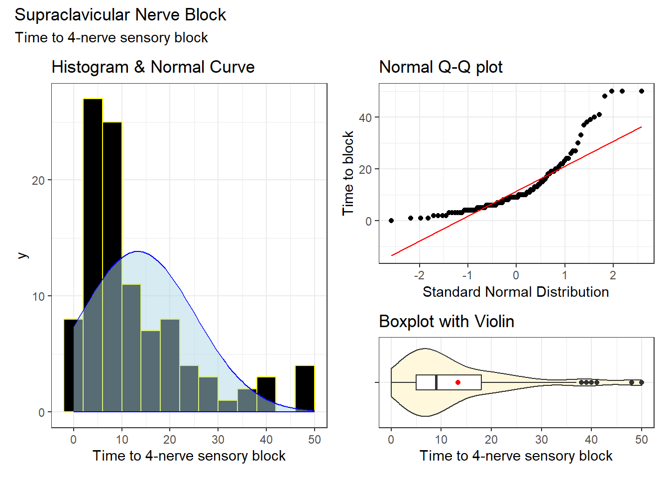
n	miss	mean	sd	med	mad	min	q25	q75	max
103	0	13.32	11.87	9	7.41	0	5	18	50

16.3.1 Log transformation of outcome

Given the apparent right skew in this outcome, let’s consider a transformation, specifically the logarithm.

supra |> reframe(lovedist(log(onset_sensory))) |>
  kable(digits = 2)

n	miss	mean	sd	med	mad	min	q25	q75	max
103	0	-Inf	NaN	2.2	0.87	-Inf	1.61	2.89	3.91

Oh, yes, we need to do something about the minimum value in the original onset_sensory data being zero, instead of a positive number.

Let’s try this:

supra <- supra |>
  mutate(os_tr = log(onset_sensory + 1))

supra |> reframe(lovedist(os_tr)) |>
  kable(digits = 2)

n	miss	mean	sd	med	mad	min	q25	q75	max
103	0	2.35	0.8	2.3	0.76	0	1.79	2.94	3.93

We’ll need to select a new bin width for the histogram as well. A little experimenting suggests 0.2 as a choice that produces an attractive histogram, where the overlaid Normal distribution is also clear.

bw = 0.2 # specify width of bins in histogram

p1t <- ggplot(supra, aes(os_tr)) +
  geom_histogram(binwidth = bw, 
                 fill = "black", col = "yellow") +
  stat_function(fun = function(x)
    dnorm(x, mean = mean(supra$os_tr, 
                         na.rm = TRUE),
          sd = sd(supra$os_tr, 
                  na.rm = TRUE)) *
      length(supra$os_tr) * bw,  
    geom = "area", alpha = 0.5,
    fill = "lightblue", col = "blue"
    ) +
  labs(
    x = "log(Time to 4-nerve sensory block + 1)",
    title = "Histogram & Normal Curve"
  ) 

p2t <- ggplot(supra, aes(sample = os_tr)) +
  geom_qq() +
  geom_qq_line(col = "red") +
  labs(
    y = "log(Time to block + 1)",
    x = "Standard Normal Distribution",
    title = "Normal Q-Q plot"
  ) 

p3t <- ggplot(supra, aes(x = os_tr, y = "")) +
  geom_violin(fill = "cornsilk") +
  geom_boxplot(width = 0.2) +
  stat_summary(
    fun = mean, geom = "point",
    shape = 16, col = "red"
  ) +
  labs(
    y = "", x = "log(Time to block + 1)",
    title = "Boxplot with Violin"
  ) 

p1t + (p2t / p3t + plot_layout(heights = c(2, 1))) +
  plot_annotation(
    title = "Supraclavicular Nerve Block",
    subtitle = "log(Time to 4-nerve sensory block + 1)"
  )

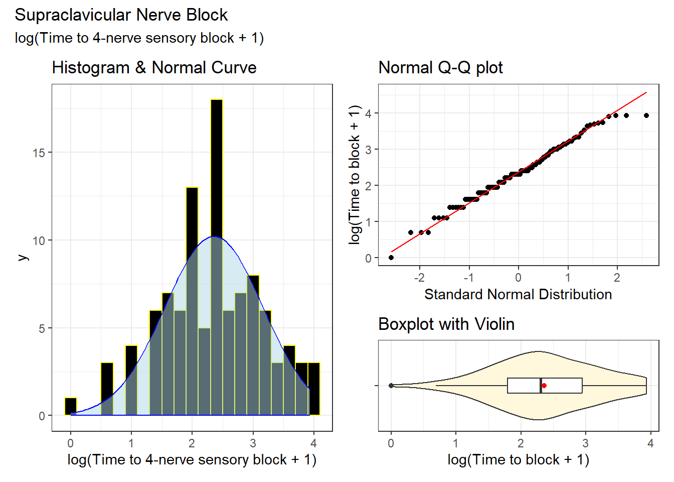
This looks like a fairly promising outcome variable for a linear model, with a distribution that can be well-approximated by the Normal distribution.

16.4 Time to Block by Group

Let’s investigate the impact of group (either sequential or mixture) on our transformed outcome, log(onset_sensory + 1).

16.4.1 Least Squares Linear Model

fit1 <- lm(os_tr ~ group, data = supra)

model_parameters(fit1, ci = 0.95)

Parameter          | Coefficient |   SE |       95% CI | t(101) |      p
------------------------------------------------------------------------
(Intercept)        |        2.17 | 0.11 | [1.95, 2.38] |  19.89 | < .001
group [Sequential] |        0.38 | 0.15 | [0.07, 0.68] |   2.43 | 0.017 

Uncertainty intervals (equal-tailed) and p-values (two-tailed) computed
  using a Wald t-distribution approximation.

Of course, this is just a two-sample t test assuming equal variances, which yields a confidence interval for the difference in population means of our transformed outcome.

If we compare two patients, one assigned to the mixture group and one assigned to the sequential group, our model estimates that, on average, the subject assigned to the sequential group will have a log(time to 4-nerve sensory block onset + 1) value that is 0.38 longer than the subject assigned to the mixture group. The 95% confidence interval around that point estimate is (0.07, 0.68.)

Each of the values in the CI are consistent with the notion that the mixture group patients had lower times (as well as lower log(time + 1) values) than did the sequential group. This is because within the range of onset times we observed, the logarithm does not change the order when we compare two subjects.

It’s not strictly necessary when we compare two groups like this, but we can estimate the difference in our transformed outcome across the groups with estimate_contrasts() as well, like this.

estimate_contrasts(fit1, contrast = "group")

Marginal Contrasts Analysis

Level1  |     Level2 | Difference |         95% CI |   SE | t(101) |     p
--------------------------------------------------------------------------
Mixture | Sequential |      -0.38 | [-0.68, -0.07] | 0.15 |  -2.43 | 0.017

Marginal contrasts estimated at group
p-value adjustment method: Holm (1979)

Note the sign flip to show the mixture - sequential difference.

Since we’ve used a logarithm here, it is appealing to consider presenting the resulting difference in terms of a multiplicative effect on the original data. Here, of course, we had to add 1 (or some other constant) to each onset sensory time to be able to use a logarithm.

In our model, a one-unit difference (from sensory to mixture) results in a 0.38 difference in the log of (onset sensory time + 1). This means that such a difference results in a multiplicative factor of \(exp(0.38) = 1.46\). Exponentiating the confidence interval for our transformed outcome we get \(exp(0.07) = 1.07\) and \(exp(0.68) = 1.97\).

So, another way to describe our result is as follows:

If we compare two patients, one assigned to the mixture group and one assigned to the sequential group, our model estimates that, on average, the subject assigned to the sequential group will have a (time to 4-nerve sensory block onset + 1) value that is 1.46 times that of the subject assigned to the mixture group. The 95% confidence interval around that point estimate is (1.07, 1.97).

Now, since all of the values in that exponentiated confidence interval exceed 1, they are consistent with the notion that the sequential group patients had longer times to onset than did the mixture group.

How well does our model perform?

model_performance(fit1)

# Indices of model performance

AIC     |    AICc |     BIC |    R2 | R2 (adj.) |  RMSE | Sigma
---------------------------------------------------------------
246.725 | 246.967 | 254.629 | 0.055 |     0.046 | 0.779 | 0.786

It appears that this model accounts for about 5.5% of the variation in our transformed outcome.

We can look at the full set of residual plots, but they’re not so helpful in this case where we only have a single categorical predictor (and with only two categories.) The most directly relevant plots are those we built in prior chapters to look at the assumptions of equal variance and normality across our two groups, for example the plot below which shows similar variation and no strong skew or especially problematic outliers across the transformed times in our two exposure groups.

ggplot(data = supra, aes(x = group, y = os_tr)) +
  geom_violin() +
  geom_boxplot(width = 0.3) +
  stat_summary(fun = "mean", col = "red", geom = "point")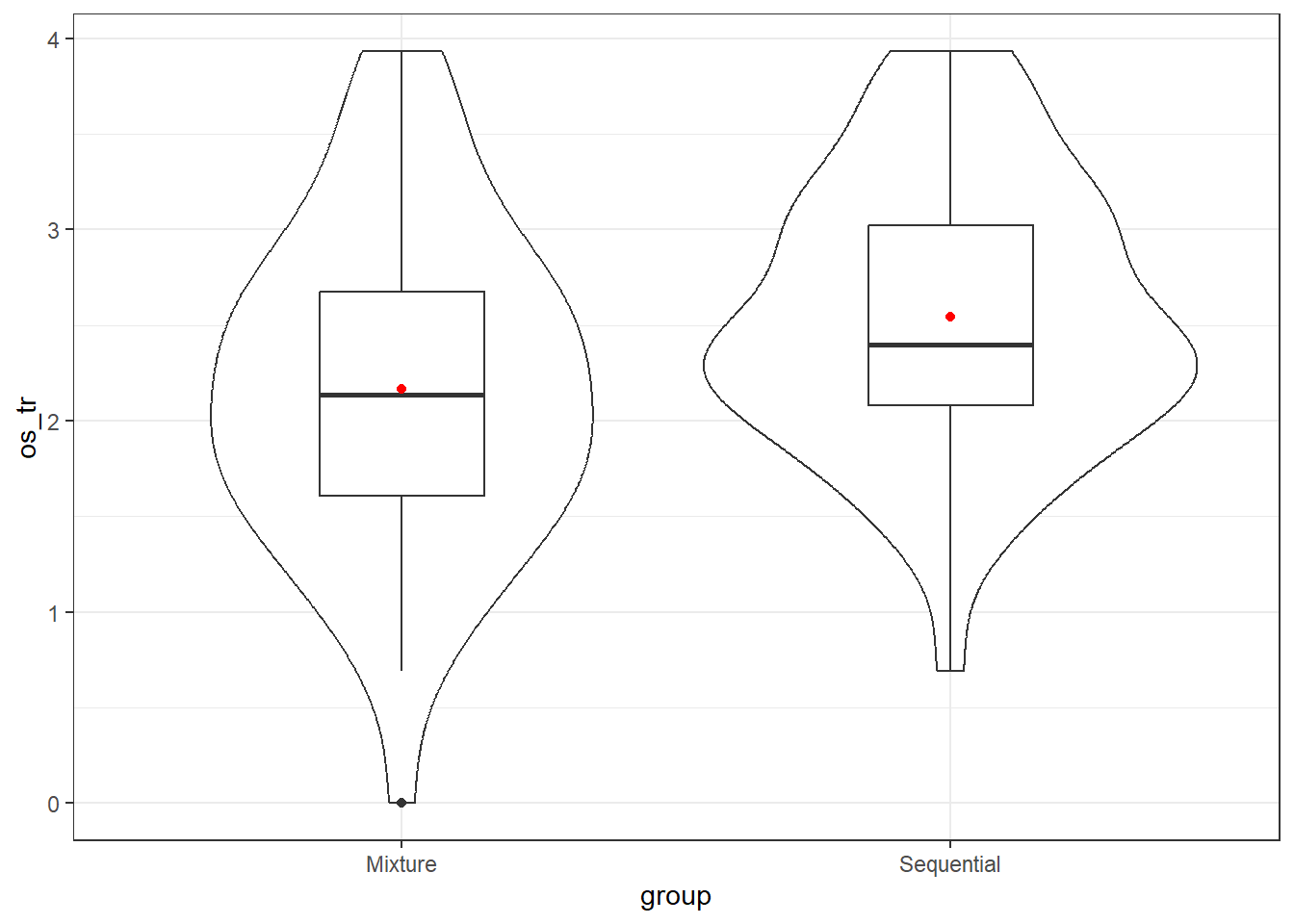

As mentioned, we can run the full spectrum of residual plots with check_model(fit1) but I would focus on just two of the plots whenever I have only one predictor and it is categorical, specifically the plots of

• posterior predictive checks, and
• normality of residuals

as shown below.

check_predictions(fit1)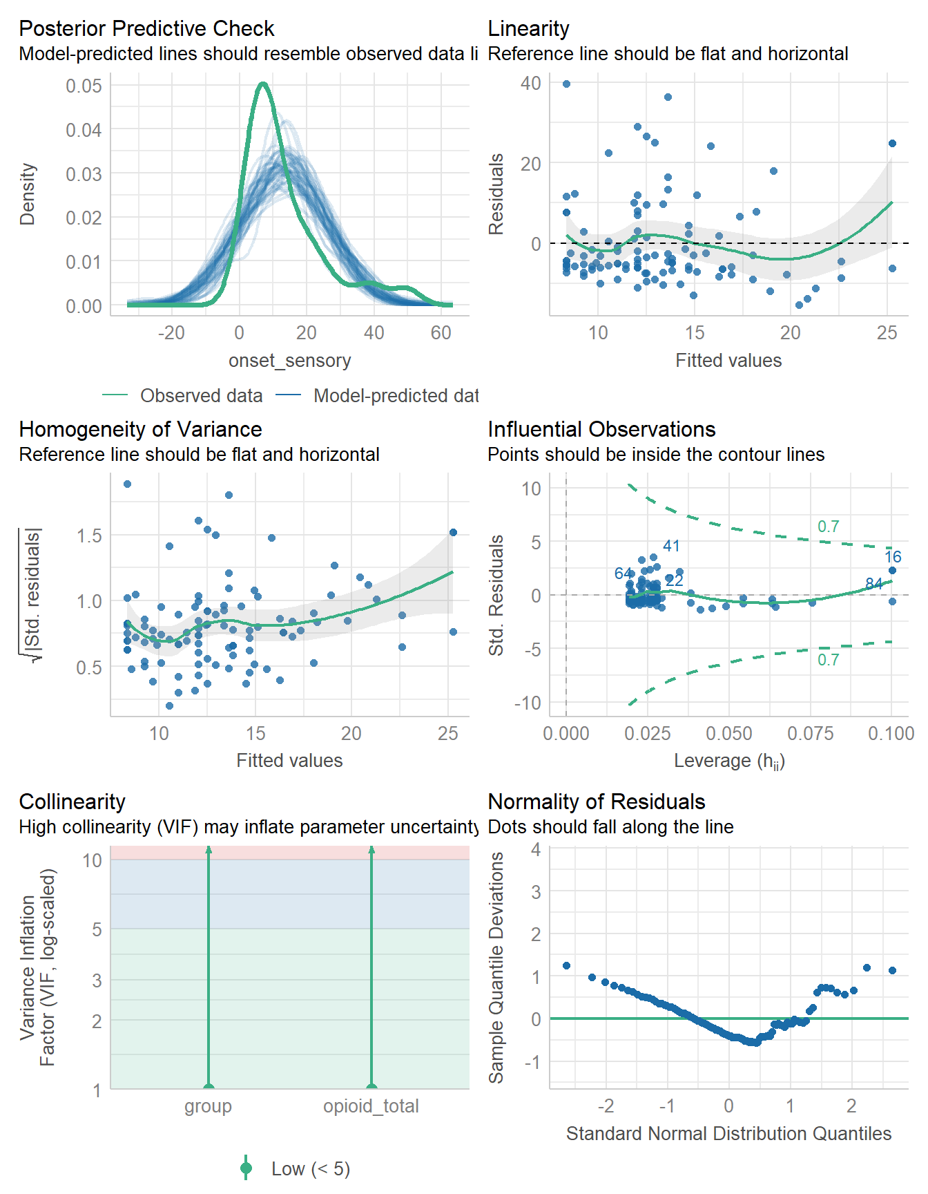

I see no substantial problems here. The model-predicted data seem to (mostly) cluster around the reference curve for the observed data.

plot(check_normality(fit1))

For confidence bands, please install `qqplotr`.

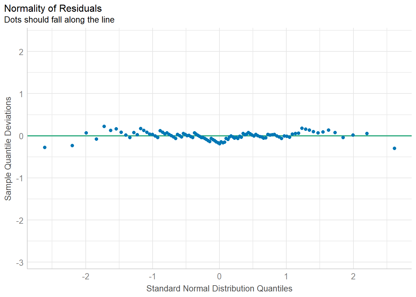
Again, there’s no real problem here with the assumption of Normality as shown in this detrended Normal Q-Q plot. The points fall close to the reference line.

16.4.2 Bayesian linear model

Let us instead fit a Bayesian model (with a weakly informative prior, as usual) to our transformed outcome, and see if this yields a meaningfully different set of estimates.

set.seed(431)
fit2 <- stan_glm(os_tr ~ group, data = supra, refresh = 0)

model_parameters(fit2, ci = 0.95)

Parameter       | Median |       95% CI |     pd |  Rhat |     ESS |                 Prior
------------------------------------------------------------------------------------------
(Intercept)     |   2.17 | [1.94, 2.39] |   100% | 1.000 | 3899.00 | Normal (2.35 +- 2.01)
groupSequential |   0.37 | [0.06, 0.70] | 99.05% | 1.000 | 3793.00 | Normal (0.00 +- 4.00)

estimate_contrasts(fit2, contrast = "group")

Marginal Contrasts Analysis

Level1  |     Level2 | Difference |         95% CI |     pd | % in ROPE
-----------------------------------------------------------------------
Mixture | Sequential |      -0.37 | [-0.70, -0.06] | 99.05% |     1.84%

Marginal contrasts estimated at group

The estimates are almost the same as those we saw in our linear model fit with OLS, and this is unsurprising, given our choice of an automated weakly informative prior.

Again, the model suggests that on average, the sequential group had longer onset times than the mixture group.

model_performance(fit2)

# Indices of model performance

ELPD     | ELPD_SE |   LOOIC | LOOIC_SE |    WAIC |    R2 | R2 (adj.) |  RMSE | Sigma
-------------------------------------------------------------------------------------
-123.468 |   7.070 | 246.937 |   14.139 | 246.918 | 0.053 |     0.026 | 0.779 | 0.791

The model performance for this fit suggests that we have now accounted for 5.3% of the variation in our outcome, so that’s a slight drop from the OLS fit (fit1). How are the predictions?

check_predictions(fit2)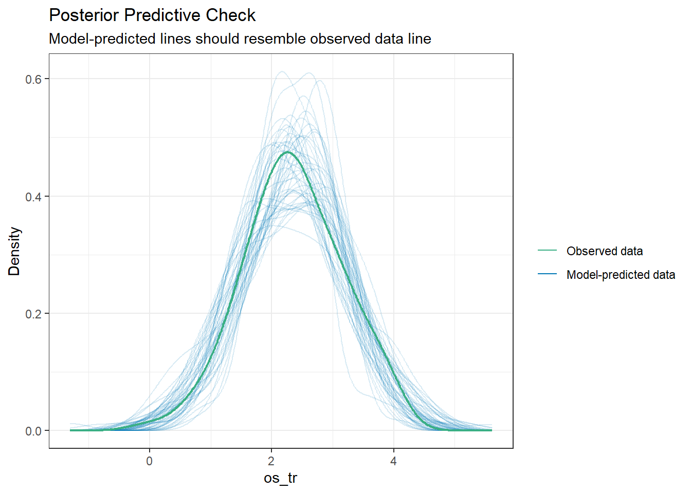

Again, the predictions from the model seem reasonably close in distribution to the observed data. So we have two models (one with OLS, one with Bayes) for our transformed outcome which are similar in what they suggest and their quality of fit.

16.5 Adjusting for Opioid Consumption

As we discussed earlier, we want to consider whether the comparison of onset times across our two groups (sequential and mixture) would be more helpful if we used our model to also account for an important covariate. Covariates are typically quantitative measures (here, we are looking at opioid consumption, in mg) obtained prior to the exposure decision.

16.5.1 Least Squares Linear Model

Let’s fit the OLS model, now including opioid consumption as a predictor along with our group variable, still for our transformed outcome.

fit3 <- lm(os_tr ~ group + opioid_total, data = supra)

model_parameters(fit3, ci = 0.95)

Parameter          | Coefficient |       SE |       95% CI | t(100) |      p
----------------------------------------------------------------------------
(Intercept)        |        1.94 |     0.12 | [1.70, 2.19] |  15.89 | < .001
group [Sequential] |        0.37 |     0.15 | [0.07, 0.66] |   2.49 | 0.014 
opioid total       |    4.30e-03 | 1.24e-03 | [0.00, 0.01] |   3.46 | < .001

Uncertainty intervals (equal-tailed) and p-values (two-tailed) computed
  using a Wald t-distribution approximation.

To interpret these results, we have to constrain our comparison a bit further than we did originally. Specifically, our model’s estimates now compare two patients with the same opioid consumption who differ in terms of the anesthetic group (one in sequential, the other in mixture.) Our model estimates that, on average, the subject assigned to the sequential group will have a log(time to 4-nerve sensory block onset + 1) value that is 0.37 longer than the subject assigned to the mixture group who has the same level of opioid consumption. The 95% confidence interval around that point estimate is (0.07, 0.66.) So our estimate for the group effect remains close to the original value (0.38) at 0.37, with a similar confidence interval of (0.07, 0.66) to what we saw previously, even after adjusting for opioid consumption.

The important difference between the two models is that by adjusting for opioid consumption, we have accounted for a much larger proportion of the variation in our outcome with our model fit3 than we did with either of our models that ignored opioid consumption.

model_performance(fit3)

# Indices of model performance

AIC     |    AICc |     BIC |    R2 | R2 (adj.) |  RMSE | Sigma
---------------------------------------------------------------
237.058 | 237.466 | 247.597 | 0.156 |     0.139 | 0.736 | 0.747

We see that our \(R^2\) value has increased to 15.6% of the variation in our transformed outcome, as compared to the 5.5% we saw in the model without opioid consumption.

How about the residual plots?

• Note that here I’m running the complete set of plots, since I have at least one quantitative predictor (opioid consumption) in model fit3.

check_model(fit3)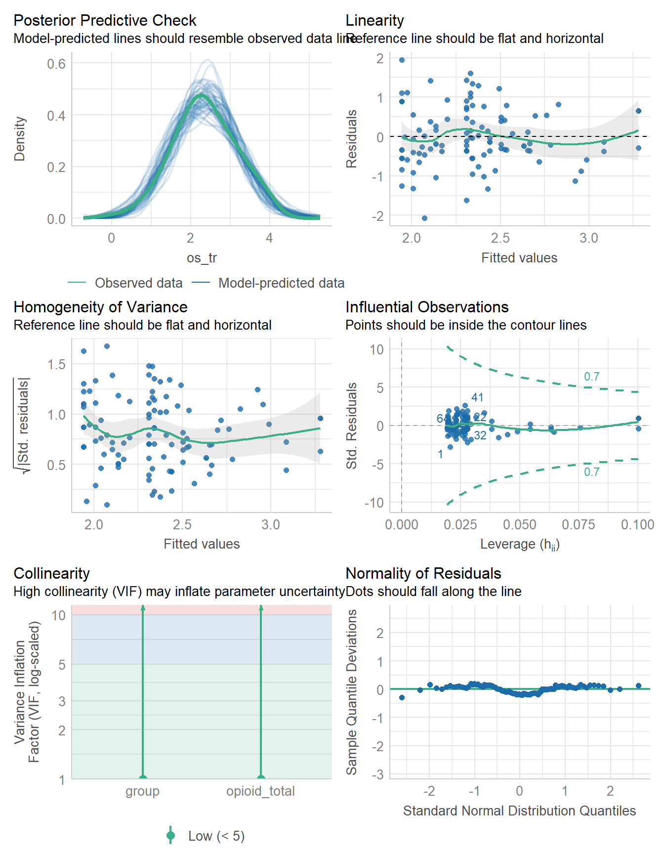

The plots describing posterior predictive checks and the Normality of our model’s residuals look about as good as they did before, and we have no new strong problems with the assumptions of linearity or constant variance, as well as no points that appear particularly influential.

The new plot (obtained when we fit a regression model with multiple predictors) is a plot related to collinearity and the variance inflation factor. We will address this in later work. For now, we seem to have a reasonable model, although not a particularly strong one (since the model \(R^2\) is fairly low.)

16.5.2 Bayesian linear model

Do we get meaningfully different results with a Bayesian fit here? Essentially, no.

set.seed(431)
fit4 <- stan_glm(os_tr ~ group + opioid_total, 
                 data = supra, refresh = 0)

model_parameters(fit4, ci = 0.95)

Parameter       |   Median |       95% CI |     pd |  Rhat |     ESS |                 Prior
--------------------------------------------------------------------------------------------
(Intercept)     |     1.94 | [1.70, 2.18] |   100% | 1.000 | 5150.00 | Normal (2.35 +- 2.01)
groupSequential |     0.37 | [0.09, 0.65] | 99.40% | 1.001 | 4566.00 | Normal (0.00 +- 4.00)
opioid_total    | 4.28e-03 | [0.00, 0.01] | 99.98% | 1.000 | 5144.00 | Normal (0.00 +- 0.03)

estimate_contrasts(fit4, contrast = "group")

Marginal Contrasts Analysis

Level1  |     Level2 | Difference |         95% CI |     pd | % in ROPE
-----------------------------------------------------------------------
Mixture | Sequential |      -0.37 | [-0.65, -0.09] | 99.40% |     0.87%

Marginal contrasts estimated at group

model_performance(fit4)

# Indices of model performance

ELPD     | ELPD_SE |   LOOIC | LOOIC_SE |    WAIC |    R2 | R2 (adj.) |  RMSE | Sigma
-------------------------------------------------------------------------------------
-118.500 |   7.349 | 237.001 |   14.698 | 236.973 | 0.160 |     0.117 | 0.736 | 0.748

check_model(fit4)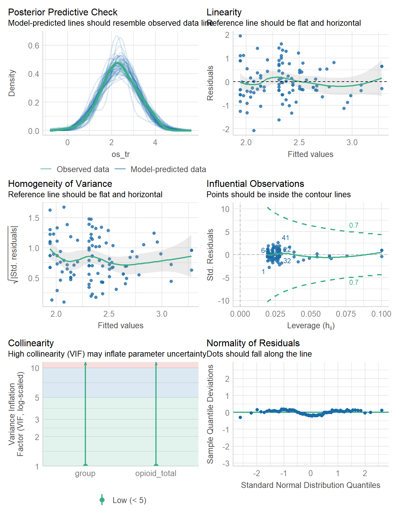

The estimates, residual plots, posterior predictive check and model performance summaries that we can compare between our OLS fit3 and our Bayesian fit4 all look quite similar. We’ll leave that there for now.

16.6 For More Information

Chapters 7, 8, 24 and 25 of Introduction to Modern Statistics Çetinkaya-Rundel and Hardin (2024) are useful here.

Çetinkaya-Rundel, Mine, and Johanna Hardin. 2024. Introduction to Modern Statistics. Second Edition. OpenIntro Project. https://openintro-ims.netlify.app/.

Higgins, Peter. 2023. “Medicaldata: Data Package for Medical Datasets.” https://higgi13425.github.io/medicaldata/.

Roberman, Dmitry, Harendra Arora, Daniel I. Sessler, Michael Ritchey, Jing You, and Priya Kumar. 2011. “Combined Versus Sequential Injection of Mepivacaine and Ropivacaine for Supraclavicular Nerve Blocks.” Reg Anesth Pain Med 36: 145–50.

---

1. Supraclavicular refers to the area above the clavicle, or collarbone, on either side of the body.

2. Onset_first_sensory was defined as time from the completion of anesthetic injection until development of first sensory block to sharp pain.

3. Two subjects (subjects 16 and 84) failed to achieve complete sensory and motor block, and these were censored at 50 minutes. We’ll ignore this here.