17 Missing Data and World Nations
17.1 R setup for this chapter
Appendix A lists all R packages used in this book, and also provides R session information. Appendix B describes the 431-Love.R script, and demonstrates its use.
17.2 Data on Nations of the World
Appendix C provides further guidance on pulling data from other systems into R, while Appendix D gives more information (including download links) for all data sets used in this book.
I collected these data from the World Health Organization and other sources, as of the end of May 2024. The primary resource was the Global Health Observatory from the WHO. Other resources included:
- The World Health Statistics Report
- Table of World Health Statistics 2024
- Gross Domestic Product Per Capita comes from the World Bank, accessed 2024-06-20.
nations <- read_csv("data/nations.csv", show_col_types = FALSE) |>
  mutate(
    UNIV_CARE = factor(UNIV_CARE),
    WHO_REGION = factor(WHO_REGION),
    C_NUM = as.character(C_NUM),
    GDP_PERCAP = GDP_PERCAP/1000
  ) |>
  janitor::clean_names()

glimpse(nations)
Rows: 192
Columns: 7
$ c_num <chr> "1", "2", "3", "4", "5", "6", "7", "8", "9", "10", "11", …
$ country_name <chr> "Afghanistan", "Albania", "Algeria", "Andorra", "Angola",…
$ iso_alpha3 <chr> "AFG", "ALB", "DZA", "AND", "AGO", "ATG", "ARG", "ARM", "…
$ uhc_index <dbl> 41, 64, 74, 79, 37, 76, 79, 68, 87, 85, 66, 77, 76, 52, 7…
$ univ_care <fct> no, yes, yes, no, no, no, yes, no, yes, yes, no, yes, no,…
$ gdp_percap <dbl> 0.356, 6.810, 4.343, 41.993, 3.000, 19.920, 13.651, 7.018…
$ who_region <fct> Eastern Mediterranean, European, African, European, Afric…The data include information on 7 variables (listed below), describing 192 separate countries of the world.
By Country, we mean a sovereign state that is a member of both the United Nations and the World Health Organization, in its own right. Note that Liechtenstein is not a member of the World Health Organization, but is in the UN. Liechtenstein is the only UN member nation not included in the nations data.
| Variable | Description |
|---|---|
c_num |
Country ID (alphabetical by country_name) |
country_name |
Name of Country (according to WHO and UN) |
iso_alpha3 |
ISO Alphabetical 3-letter code gathered from WHO |
uhc_index |
Universal Health Coverage: Service coverage index1 - higher numbers indicate better coverage. |
univ_care |
Yes if country offers government-regulated and government-funded health care to more than 90% of its citizens as of 2023, else No |
gdp_percap |
GDP Per Capita per the World Bank in thousands of 2023 US dollars2 |
who_region |
Six groups3 according to regional distribution |
17.3 Exploratory Data Analysis
Our interest is in understanding the association of uhc_index and univ_care, perhaps after adjustment for the country’s gdp_percap.
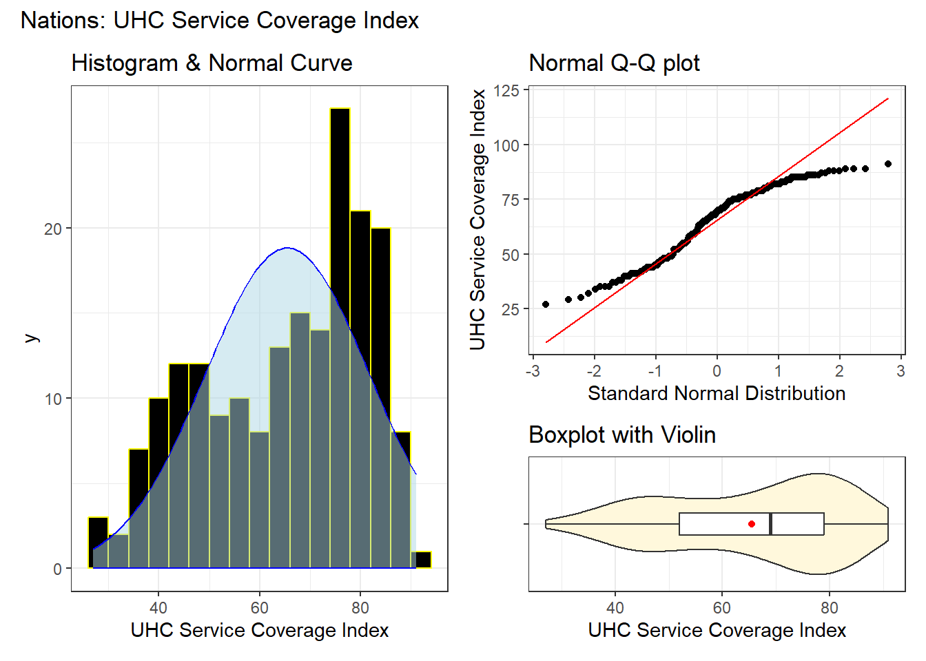
17.3.1 EDA for our outcome
bw = 4 # specify width of bins in histogram

p1 <- ggplot(nations, aes(uhc_index)) +
  geom_histogram(binwidth = bw,
                 fill = "black", col = "yellow") +
  stat_function(fun = function(x)
    dnorm(x, mean = mean(nations$uhc_index,
                         na.rm = TRUE),
          sd = sd(nations$uhc_index,
                  na.rm = TRUE)) *
      length(nations$uhc_index) * bw,
    geom = "area", alpha = 0.5,
    fill = "lightblue", col = "blue"
    ) +
  labs(
    x = "UHC Service Coverage Index",
    title = "Histogram & Normal Curve"
  )

p2 <- ggplot(nations, aes(sample = uhc_index)) +
  geom_qq() +
  geom_qq_line(col = "red") +
  labs(
    y = "UHC Service Coverage Index",
    x = "Standard Normal Distribution",
    title = "Normal Q-Q plot"
  )

p3 <- ggplot(nations, aes(x = uhc_index, y = "")) +
  geom_violin(fill = "cornsilk") +
  geom_boxplot(width = 0.2) +
  stat_summary(
    fun = mean, geom = "point",
    shape = 16, col = "red"
  ) +
  labs(
    y = "", x = "UHC Service Coverage Index",
    title = "Boxplot with Violin"
  )

p1 + (p2 / p3 + plot_layout(heights = c(2, 1))) +
  plot_annotation(
    title = "Nations: UHC Service Coverage Index"
  )
17.3.2 UHC Service Coverage by Universal Care Status
ggplot(nations, aes(y = univ_care, x = uhc_index,
                    fill = univ_care)) +
  geom_violin() +
  geom_boxplot(width = 0.3, fill = "cornsilk", notch = TRUE) +
  stat_summary(fun = mean, geom = "point", fill = "red",
               size = 3, shape = 21) +
  scale_fill_brewer(palette = "Set2") +
  guides(fill = "none")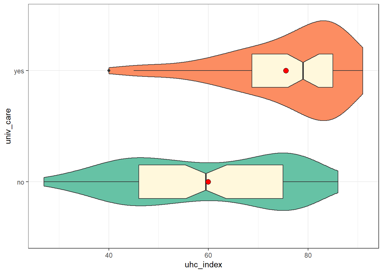
17.3.3 Per-capita GDP
Shortly, we’ll fit models including per-capita GDP. Can we summarize that data, too?
| n | miss | mean | sd | med | mad | min | q25 | q75 | max |
|---|---|---|---|---|---|---|---|---|---|
| 192 | 4 | 17.42 | 27.95 | 6.7 | 7.9 | 0.26 | 2.26 | 20.24 | 240.86 |
ggplot(nations, aes(y = univ_care, x = gdp_percap)) +
  geom_boxplot(width = 0.3, fill = "cornsilk") +
  stat_summary(fun = mean, geom = "point", fill = "red",
               size = 3, shape = 21)
Warning: Removed 4 rows containing non-finite outside the scale range
(`stat_boxplot()`).Warning: Removed 4 rows containing non-finite outside the scale range
(`stat_summary()`).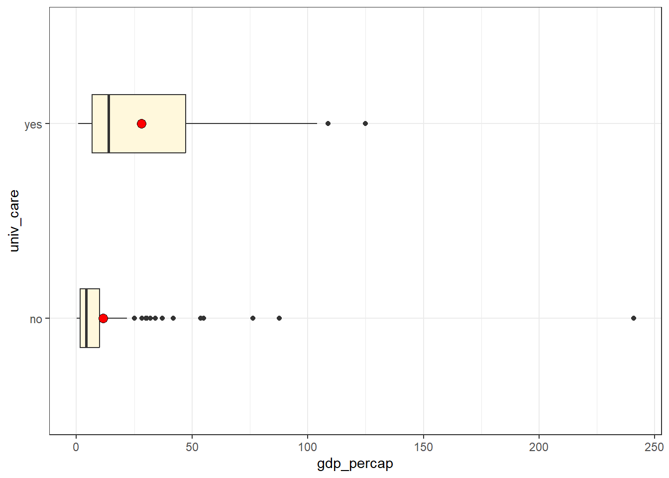
We receive a warning that we are missing four values of gdp_percap, and we also see some enormous right skew within each group, including a huge outlier at a gdp_percap near 240. Which nation is that?
nations |> filter(gdp_percap > 200)# A tibble: 1 × 7
c_num country_name iso_alpha3 uhc_index univ_care gdp_percap who_region
<chr> <chr> <chr> <dbl> <fct> <dbl> <fct>
1 112 Monaco MCO 86 no 241. European It’s Monaco. We may want to remember that.
17.4 Should we transform our outcome?
Eventually, we will consider including the gdp_percap predictor in our model, so let’s include that here, as well as univ_care when predicting uhc_index.
fit1 <- lm(uhc_index ~ univ_care + gdp_percap,
           data = nations)

boxCox(fit1, main = "Transforming UHC_Index")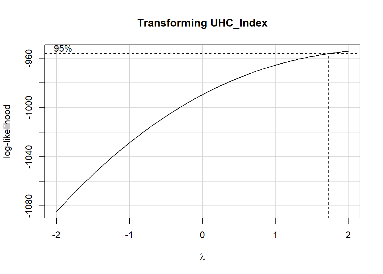
summary(powerTransform(fit1))$result Est Power Rounded Pwr Wald Lwr Bnd Wald Upr Bnd
Y1 2.532079 2 1.908487 3.15567117.4.1 Looking at Residual Plots
We might consider whether the residuals from our two models (with and without transforming the outcome) follow the assumption of a Normal distribution.
Here, I’ve decided to scale the squared values of uhc_index into normal deviates, by centering them (subtracting their mean) and scaling them (dividing by their standard deviation). The value of centering and scaling here is to avoid huge predictions, and to generate residuals that should have a mean of 0 and standard deviation of 1.
fit2 <- lm(scale(uhc_index^2, center = TRUE, scale = TRUE) ~
             univ_care + gdp_percap,
           data = nations)

resids_df <- tibble(raw = fit1$residuals,
                 sqr = fit2$residuals)

p1 <- ggplot(resids_df, aes(sample = raw)) +
  geom_qq() + geom_qq_line(col = "red") +
  labs(title = "uhc_index",
       subtitle = "Normal Q-Q for fit1 residuals")

p2 <- ggplot(resids_df, aes(sample = sqr)) +
  geom_qq() + geom_qq_line(col = "red") +
  labs(title = "Scaled Square of uhc_index",
       subtitle = "Normal Q-Q for fit2 residuals")

p1 + p2 +
  plot_annotation("How well do we support a Normality assumption?")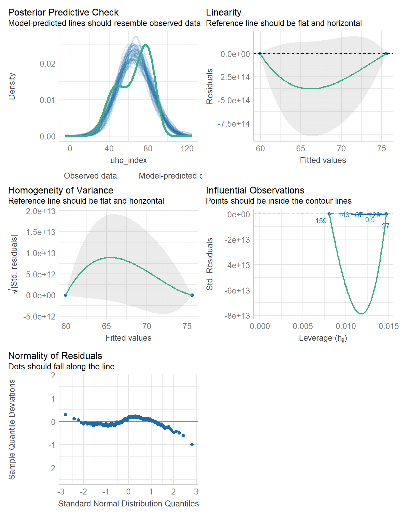
In terms of providing a better match to the assumption of Normality in the residuals, the square transformation doesn’t appear to be very helpful. If anything, our problem with light tails (fewer values far from the mean than expected) may get a little worse in fit2. So we’ll skip the transformation and work with our original outcome in what follows.
17.5 Least Squares Linear Model
fit3 <- lm(uhc_index ~ univ_care, data = nations)

model_parameters(fit3, ci = 0.95)
Parameter | Coefficient | SE | 95% CI | t(190) | p
-----------------------------------------------------------------------
(Intercept) | 59.92 | 1.30 | [57.35, 62.49] | 46.04 | < .001
univ care [yes] | 15.65 | 2.19 | [11.34, 19.97] | 7.16 | < .001
Uncertainty intervals (equal-tailed) and p-values (two-tailed) computed
using a Wald t-distribution approximation.estimate_contrasts(fit3, contrast = "univ_care", ci = 0.95)Marginal Contrasts Analysis
Level1 | Level2 | Difference | 95% CI | SE | t(190) | p
------------------------------------------------------------------------
no | yes | -15.65 | [-19.97, -11.34] | 2.19 | -7.16 | < .001
Marginal contrasts estimated at univ_care
p-value adjustment method: Holm (1979)17.5.1 Interpreting the Fit
Here are two equivalent interpretations:
- When comparing two nations where one offers universal health care and the other does not, the country that offers universal care will, on average, have a UHC index score that is 15.7 points higher (with 95% CI 11.34, 19.97) points.
- Under this fitted model, the average difference in UHC index score between a country that offers universal health care and one that does not is 15.7 points (95% uncertainty interval for the estimated difference is 11.34, 19.97 points.)
17.5.2 Performance of the Model
model_performance(fit3)# Indices of model performance
AIC | AICc | BIC | R2 | R2 (adj.) | RMSE | Sigma
--------------------------------------------------------------------
1575.544 | 1575.672 | 1585.317 | 0.212 | 0.208 | 14.417 | 14.493The model accounts for 21.2% of the variation in our uhc_index outcome.
17.5.3 Checking the Model
Again, since our fit3 model here is just a two-sample t test, we’ll focus on two plots, rather than the whole set.
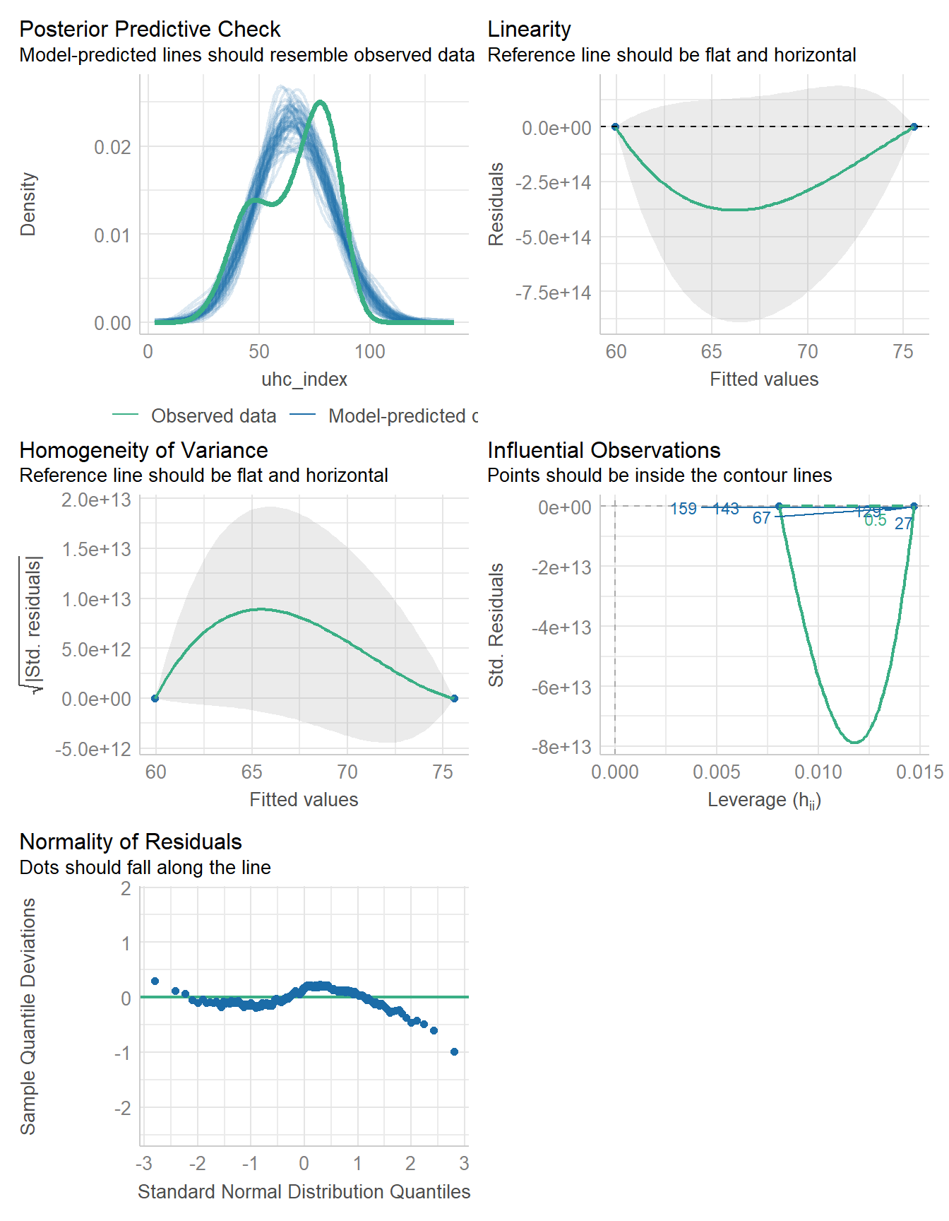
Now we seem to have a real problem with our posterior predictive checks. The observed data shows two modes (one near 50 and one near 80) which our model-simulated results are completely missing. The assumption of Normality continues to be an issue, as well.
A Bayesian fit of this model with a weakly informative prior continues to show the same problems, although I’ll spare you that output here.
17.6 Missing Data Mechanisms
We now tackle the issue of missing data.
My source for the following description of mechanisms is Chapter 25 of Gelman and Hill (2007), and that chapter is available at this link.
-
MCAR = Missingness completely at random. A variable is missing completely at random if the probability of missingness is the same for all units, for example, if for each subject, we decide whether to collect
gdp_percapby rolling a die and refusing to answer if a “6” shows up. If data are missing completely at random, then throwing out cases with missing data does not bias your inferences.
We have tacitly made the MCAR assumption in all of our prior dealings with missing data in this book.
Missingness that depends only on observed predictors. A more general assumption, called missing at random or MAR, is that the probability a variable is missing depends only on available information. Here, we would have to be willing to assume that the probability of non-response to
gdp_percapdepends only on the other, fully recorded variables in the data. It is often reasonable to model this process as a logistic regression, where the outcome variable equals 1 for observed cases and 0 for missing. When an outcome variable is missing at random, it is acceptable to exclude the missing cases (that is, to treat them as NA), as long as the regression adjusts for all of the variables that affect the probability of missingness.Missingness that depends on unobserved predictors. Missingness is no longer “at random” if it depends on information that has not been recorded and this information also predicts the missing values. If a particular treatment causes discomfort, a patient is more likely to drop out of the study. This missingness is not at random (unless “discomfort” is measured and observed for all patients). If missingness is not at random, it must be explicitly modeled, or else you must accept some bias in your inferences.
Missingness that depends on the missing value itself. Finally, a particularly difficult situation arises when the probability of missingness depends on the (potentially missing) variable itself. For example, suppose that people with higher earnings are less likely to reveal them.
Essentially, situations 3 and 4 are referred to collectively as non-random missingness, and cause more trouble for us than 1 and 2.
17.7 Ways to Deal with Missing Data
There are several available methods for dealing with missing data that are MCAR or MAR, but they basically boil down to:
- Complete Case (or Available Case) analyses
- Single Imputation
- Multiple Imputation
17.7.1 Complete Case
In Complete Case analyses, rows containing NA values are omitted from the data before analyses commence. This is the default approach for many statistical software packages, and may introduce unpredictable bias and fail to include some useful, often hard-won information.
- A complete case analysis can be appropriate when the number of missing observations is not large, and the missing pattern is either MCAR (missing completely at random) or MAR (missing at random.)
- Two problems arise with complete-case analysis:
- If the units with missing values differ systematically from the completely observed cases, this could bias the complete-case analysis.
- If many variables are included in a model, there may be very few complete cases, so that most of the data would be discarded for the sake of a straightforward analysis.
- A related approach is available-case analysis where different aspects of a problem are studied with different subsets of the data, perhaps identified on the basis of what is missing in them.
17.7.2 Single Imputation
In single imputation analyses, NA values are estimated/replaced one time with one particular data value for the purpose of obtaining more complete samples, at the expense of creating some potential bias in the eventual conclusions or obtaining slightly less accurate estimates than would be available if there were no missing values in the data.
- A single imputation can be just a replacement with the mean or median (for a quantity) or the mode (for a categorical variable.) However, such an approach, though easy to understand, underestimates variance and ignores the relationship of missing values to other variables.
- Single imputation can also be done using a variety of models to try to capture information about the NA values that are available in other variables within the data set.
- In this book, we will use the
micepackage to perform single imputations, as well as multiple imputation.
17.7.3 Multiple Imputation
Multiple imputation, where NA values are repeatedly estimated/replaced with multiple data values, for the purpose of obtaining more complete samples and capturing details of the variation inherent in the fact that the data have missingness, so as to obtain more accurate estimates than are possible with single imputation.
How many imputations?
Quoting vanBuuren at https://stefvanbuuren.name/fimd/sec-howmany.html
They take a quote from Von Hippel (2009) as a rule of thumb: the number of imputations should be similar to the percentage of cases that are incomplete. This rule applies to fractions of missing information of up to 0.5.
White, Royston, and Wood (2011) suggest these criteria provide an adequate level of reproducibility in practice. The idea of reproducibility is sensible, the rule is simple to apply, so there is much to commend it. The rule has now become the de-facto standard, especially in medical applications.
It is convenient to set m = 5 during model building, and increase m only after being satisfied with the model for the “final” round of imputation. So if calculation is not prohibitive, we may set m to the average percentage of missing data. The substantive conclusions are unlikely to change as a result of raising m beyond m = 5.
17.8 Complete Case Analysis
In our study, if we want to adjust our estimates for the impact of per-capita GDP, we must deal with the fact that these data are missing for four of the nations in our data.
miss_var_summary(nations)# A tibble: 7 × 3
variable n_miss pct_miss
<chr> <int> <num>
1 gdp_percap 4 2.08
2 c_num 0 0
3 country_name 0 0
4 iso_alpha3 0 0
5 uhc_index 0 0
6 univ_care 0 0
7 who_region 0 0 nations |> filter(is.na(gdp_percap)) |>
select(country_name, iso_alpha3, gdp_percap, uhc_index, univ_care) |>
kable()| country_name | iso_alpha3 | gdp_percap | uhc_index | univ_care |
|---|---|---|---|---|
| Democratic People’s Republic of Korea | PRK | NA | 68 | yes |
| Eritrea | ERI | NA | 45 | no |
| South Sudan | SSD | NA | 34 | no |
| Venezuela (Bolivarian Republic of) | VEN | NA | 75 | no |
We can drop all of the missing values from a data set with drop_na or with na.omit or by filtering for complete.cases. Any of these approaches produces the same result.
If we don’t do anything about missing data, and simply feed the results to the lm() or stan_glm() functions, the machine will produce a fit on the complete cases.
fit5 <- lm(uhc_index ~ univ_care + gdp_percap,
data = nations)summary(fit5)
Call:
lm(formula = uhc_index ~ univ_care + gdp_percap, data = nations)

Residuals:
    Min      1Q  Median      3Q     Max
-36.161  -9.625   1.336   9.558  19.917

Coefficients:
             Estimate Std. Error t value Pr(>|t|)
(Intercept)  57.02924    1.20223  47.436  < 2e-16 ***
univ_careyes 11.04387    1.98727   5.557 9.44e-08 ***
gdp_percap    0.27041    0.03414   7.920 2.14e-13 ***
---
Signif. codes:  0 '***' 0.001 '**' 0.01 '*' 0.05 '.' 0.1 ' ' 1

Residual standard error: 12.5 on 185 degrees of freedom
  (4 observations deleted due to missingness)
Multiple R-squared:  0.4117,    Adjusted R-squared:  0.4053
F-statistic: 64.73 on 2 and 185 DF, p-value: < 2.2e-16model_parameters(fit5, ci = 0.95)Parameter | Coefficient | SE | 95% CI | t(185) | p
-----------------------------------------------------------------------
(Intercept) | 57.03 | 1.20 | [54.66, 59.40] | 47.44 | < .001
univ care [yes] | 11.04 | 1.99 | [ 7.12, 14.96] | 5.56 | < .001
gdp percap | 0.27 | 0.03 | [ 0.20, 0.34] | 7.92 | < .001
Uncertainty intervals (equal-tailed) and p-values (two-tailed) computed
using a Wald t-distribution approximation.model_performance(fit5)# Indices of model performance
AIC | AICc | BIC | R2 | R2 (adj.) | RMSE | Sigma
--------------------------------------------------------------------
1488.247 | 1488.465 | 1501.192 | 0.412 | 0.405 | 12.402 | 12.503Note the indication that this model fit has had four observations deleted due to missingness.
Finally, we check the model, which, to be clear, has multiple problems with it.
check_model(fit5)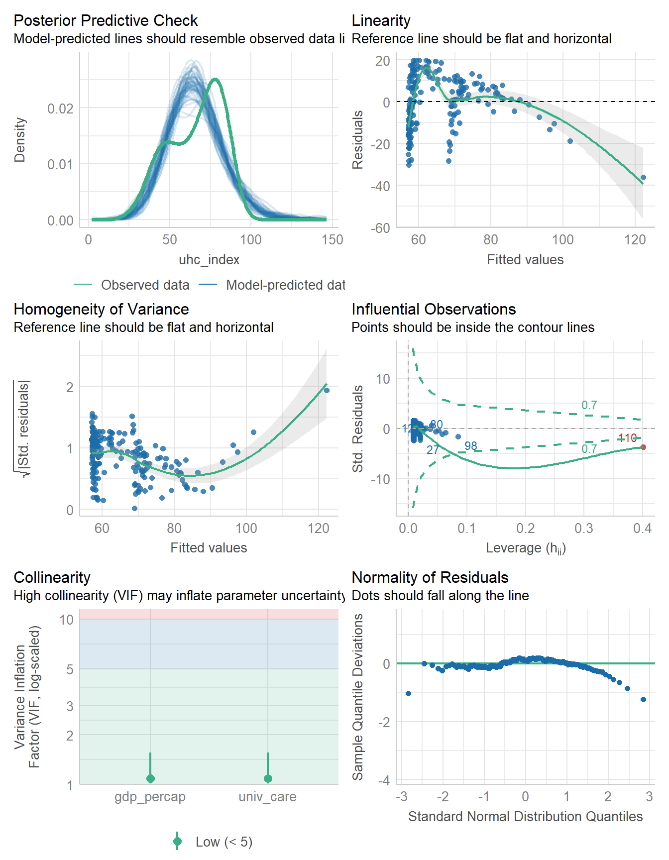
Specifically, model fit5 has problems with the posterior predictive check, the assumptions of linearity and homogeneity of variance, an influential observation, and problems with the assumption of Normality as well.
But for now, we’re not going to address any of those issues, and will instead focus on other approaches (besides complete cases) for dealing with the missing data we see in the gdp_percap data.
17.9 Single Imputation
Here is how I produced a single imputation of the nations data in R using the mice package, and some default choices, so that I could perform a regression analysis incorporating all of the nations, including those with missing gdp_percap values.
By default, mice uses predictive mean matching (or pmm), for numeric data. It uses logistic regression imputation for binary data, polytomous regression imputation for unordered categorical data with more than 2 levels, and a proportional odds regression model for ordered categorical data with more than 2 levels.
All of these methodologies will be explored in the 432 class, but a detailed explanation is beyond the scope of this book.
Warning: Number of logged events: 3Here, m is the number of imputations I want to create (here just one), seed is the random seed I set so that I can replicate the results later, and print is set to FALSE to reduce the amount of unnecessary output this produces. I will ignore this warning about logged events in most cases, including here.
If you want to see the logged events, try:
ini <- mice(nations, m = 1, seed = 431, print = FALSE)Warning: Number of logged events: 3ini$loggedEvents it im dep meth out
1 0 0 constant c_num
2 0 0 constant country_name
3 0 0 constant iso_alpha3Here, our nations data include three variables which are not included in the imputation process (and which we don’t want included) so all is well.
Here’s what I wind up with:
nations_simp# A tibble: 192 × 7
c_num country_name iso_alpha3 uhc_index univ_care gdp_percap who_region
<chr> <chr> <chr> <dbl> <fct> <dbl> <fct>
1 1 Afghanistan AFG 41 no 0.356 Eastern M…
2 2 Albania ALB 64 yes 6.81 European
3 3 Algeria DZA 74 yes 4.34 African
4 4 Andorra AND 79 no 42.0 European
5 5 Angola AGO 37 no 3 African
6 6 Antigua and Barbu… ATG 76 no 19.9 Americas
7 7 Argentina ARG 79 yes 13.7 Americas
8 8 Armenia ARM 68 no 7.02 European
9 9 Australia AUS 87 yes 65.1 Western P…
10 10 Austria AUT 85 yes 52.1 European
# ℹ 182 more rowsn_miss(nations_simp)[1] 0Now, I can do everything I did previously with this singly imputed data set.
fit6 <- lm(uhc_index ~ univ_care + gdp_percap,
data = nations_simp)summary(fit6)
Call:
lm(formula = uhc_index ~ univ_care + gdp_percap, data = nations_simp)

Residuals:
    Min      1Q  Median      3Q     Max
-36.216  -9.940   1.337   9.692  20.062

Coefficients:
             Estimate Std. Error t value Pr(>|t|)
(Intercept)  56.86773    1.19475  47.598  < 2e-16 ***
univ_careyes 11.16974    1.98286   5.633 6.34e-08 ***
gdp_percap    0.27131    0.03427   7.916 2.02e-13 ***
---
Signif. codes:  0 '***' 0.001 '**' 0.01 '*' 0.05 '.' 0.1 ' ' 1

Residual standard error: 12.59 on 189 degrees of freedom
Multiple R-squared:  0.4085,    Adjusted R-squared:  0.4023
F-statistic: 65.27 on 2 and 189 DF, p-value: < 2.2e-16model_parameters(fit6, ci = 0.95)Parameter | Coefficient | SE | 95% CI | t(189) | p
-----------------------------------------------------------------------
(Intercept) | 56.87 | 1.19 | [54.51, 59.22] | 47.60 | < .001
univ care [yes] | 11.17 | 1.98 | [ 7.26, 15.08] | 5.63 | < .001
gdp percap | 0.27 | 0.03 | [ 0.20, 0.34] | 7.92 | < .001
Uncertainty intervals (equal-tailed) and p-values (two-tailed) computed
using a Wald t-distribution approximation.model_performance(fit6)# Indices of model performance
AIC | AICc | BIC | R2 | R2 (adj.) | RMSE | Sigma
--------------------------------------------------------------------
1522.564 | 1522.778 | 1535.594 | 0.409 | 0.402 | 12.494 | 12.593And, again, we check the model, and all of the problems we have with model fit5 appear again in model fit6…
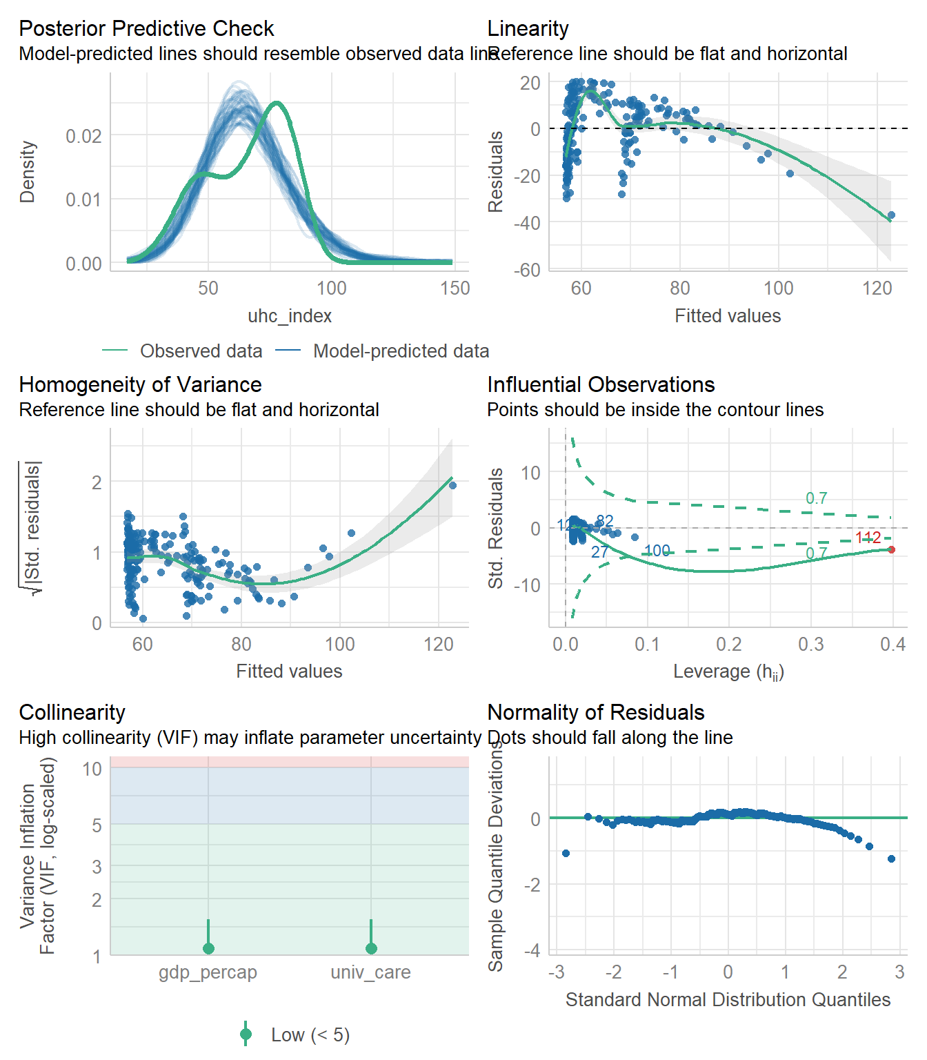
check_model(fit6)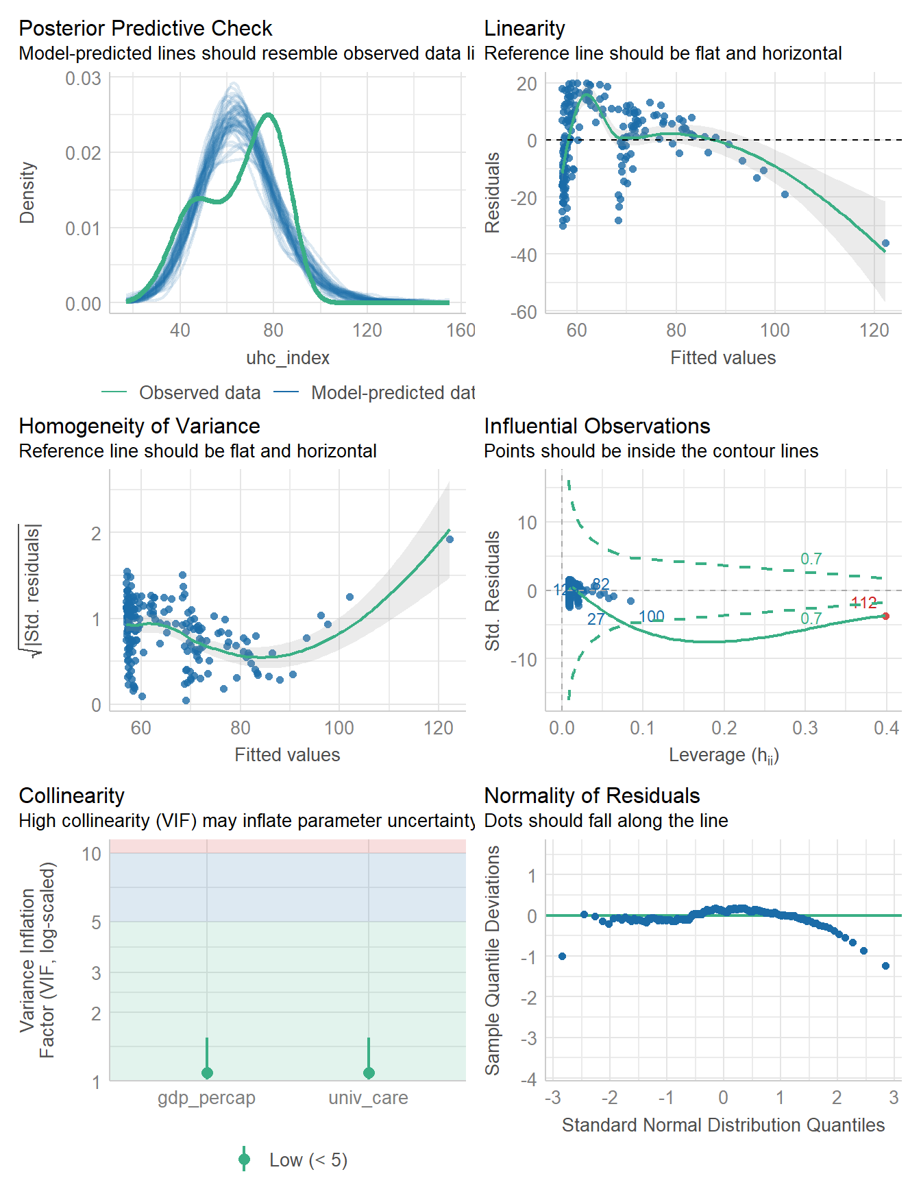
The influential point is labeled here as 112. Since we are now using the data in nations_simp to fit the model, we need to find out which country is in row 112 of that data, and it turns out to be Monaco.
slice(nations_simp, 112)# A tibble: 1 × 7
c_num country_name iso_alpha3 uhc_index univ_care gdp_percap who_region
<chr> <chr> <chr> <dbl> <fct> <dbl> <fct>
1 112 Monaco MCO 86 no 241. European 17.10 Multiple Imputation
The first thing we might consider is how many multiple imputations we want to do. Some good advice is “always do at least as many multiple imputations as the percentage of missing cases in your data” so let’s try that.
nations |> prop_miss_case()[1] 0.020833332% of the cases in our nations tibble contain missing values, so in selecting the number of imputations, I’d go for the most commonly used option, which is to use 5 imputations.
nations_imp5 <- mice(nations, m = 5, seed = 431, print = FALSE)Warning: Number of logged events: 3Here, m is the number of imputations I want to create (five, in our case), seed is the random seed I set so that I can replicate the results later, and print is set to FALSE to reduce the amount of unnecessary output this produces. I will ignore this warning about logged events in most cases, including here.
Now, we could run our model on just the first data set.
nat_imp1 <- mice::complete(nations_imp5, 1)

summary(lm(uhc_index ~ univ_care + gdp_percap, data = nat_imp1))
Call:
lm(formula = uhc_index ~ univ_care + gdp_percap, data = nat_imp1)

Residuals:
    Min      1Q  Median      3Q     Max
-36.804  -9.844   1.326   9.647  20.118

Coefficients:
             Estimate Std. Error t value Pr(>|t|)
(Intercept)  56.75761    1.19355  47.554  < 2e-16 ***
univ_careyes 11.18209    1.97351   5.666 5.38e-08 ***
gdp_percap    0.27421    0.03414   8.031 1.01e-13 ***
---
Signif. codes:  0 '***' 0.001 '**' 0.01 '*' 0.05 '.' 0.1 ' ' 1

Residual standard error: 12.55 on 189 degrees of freedom
Multiple R-squared:  0.4128,    Adjusted R-squared:  0.4066
F-statistic: 66.43 on 2 and 189 DF,  p-value: < 2.2e-16
But what we want to do is fit a set of five models, each using a different one of the five imputed data sets and obtain a summary of my results across that set of models after pooling the results, like this:
est7 <- nations |>
  mice(seed = 431, m = 5, print = FALSE) |>
  with(lm(uhc_index ~ univ_care + gdp_percap)) |>
  pool()
Warning: Number of logged events: 3model_parameters(est7, ci = 0.95)Warning: Number of logged events: 3
Warning: Number of logged events: 3
Warning: Number of logged events: 3
Warning: Number of logged events: 3# Fixed Effects
Parameter | Coefficient | SE | 95% CI | t | df | p
-------------------------------------------------------------------------------
(Intercept) | 56.81 | 1.19 | [54.46, 59.17] | 47.58 | 186.81 | < .001
univ care [yes] | 11.16 | 1.98 | [ 7.26, 15.06] | 5.64 | 187.01 | < .001
gdp percap | 0.27 | 0.03 | [ 0.21, 0.34] | 7.98 | 186.80 | < .001
Uncertainty intervals (equal-tailed) and p-values (two-tailed) computed
using a Wald t-distribution approximation.glance(est7) nimp nobs r.squared adj.r.squared
1 5 192 0.4111089 0.4048772This result looks fairly similar to my simple imputation result in terms of the coefficients and the \(R^2\) values. Unfortunately, each of my imputed data sets here has the same problems with the model as we have seen previously (as we can see below), so this isn’t an entirely satisfactory situation.
17.11 For More Information
- Chapter 25 of Gelman and Hill (2007), which is available at this link.
- See https://library.virginia.edu/data/articles/getting-started-with-multiple-imputation-in-r and the reference there to Rubin’s original work in 1976 with multiple imputation and classifying types of missing data.
- The mice package is discussed in Stef van Buuren’s book *Flexible Imputation of Missing Data, Second Edition, van Buuren (2021), available at https://stefvanbuuren.name/fimd/
This is a measure of coverage of essential health services as expressed as the average score of 14 tracer indicators of health service coverage, measured in 2021.↩︎
Some of the GDP data describes 2021, some 2022 and some 2023, depending on what was most recent and available.↩︎
The WHO regions are African, Americas, Eastern Mediterranean, European, Southeast Asian and Western Pacific.↩︎